8 Bibliotecas de R para Inferência Bayesiana
Nessa seção serão apresentadas algumas bibliotecas do R para inferência Bayesiana, em especial, LaplacesDemon e Stan, que são bibliotecas utilizadas para simular dados da posteriori. Alguns dos gráficos apresentados nessa seção serão construídos com bibliotecas específicas para avaliar amostras da posteriori, ggmcmc e bayesplot.
8.1 O Modelo de Regressão Linear
Inicialmente, será apresentado como exemplo o modelo de regressão linear, possivelmente um dos métodos mais usados nas aplicações de inferência estatística. Considere \(n\) observações de uma variável aleatória de interesse (chamada de variável dependente ou variável resposta) e de \(p-1\) características associadas a cada uma dessas observações (chamadas de variáveis dependentes ou explicativas ou covariáveis), supostamente fixadas. Um modelo de regressão linear pode ser escrito como
\[\boldsymbol{Y} = \boldsymbol{X}\boldsymbol{\beta} + \boldsymbol{\epsilon}\] com \(~\boldsymbol{Y} = \left[\begin{array}{c} Y_1\\ Y_2\\ \vdots\\ Y_n \end{array}\right]~~\); \(~~~\boldsymbol{X} = \left[\begin{array}{cccc} 1 & x_{11} & \cdots & x_{1,p-1}\\ 1 & x_{21} & \cdots & x_{2,p-1}\\ \vdots & \vdots & \ddots & \vdots \\ 1 & x_{n1} & \cdots & x_{n,p-1} \end{array}\right]~~\); \(~~~\boldsymbol{\beta} = \left[\begin{array}{c} \beta_1\\ \beta_2\\ \vdots\\ \beta_p \end{array}\right]~~\); \(~~~\boldsymbol{\epsilon} = \left[\begin{array}{c} \epsilon_1\\ \epsilon_2\\ \vdots\\ \epsilon_n \end{array}\right]~~\); \(~~~\boldsymbol{Z} = \left[\boldsymbol{X,Y}\right]~~\),
em que \(\boldsymbol{Z}\) é a matriz de dados (observada), \(\boldsymbol{\beta}\) é o vetor de parâmetros e \(\epsilon_i\) é o “erro aleatório” associado a \(i\)-ésima observação, supostamente c.i.i.d. com distribuição \(\textit{Normal}(0,\sigma^2)\).
De forma equivalente, o modelo pode ser escrito como \(\boldsymbol{Y}|\boldsymbol{X},\boldsymbol{\beta},\sigma \sim \textit{Normal}_{~n}(\boldsymbol{\mu},\boldsymbol{\Sigma})\) com \(\boldsymbol{\mu}=\boldsymbol{X}\boldsymbol{\beta}\) e \(\boldsymbol{\Sigma}=\sigma^2\boldsymbol{I}\).
\(~\)
Na abordagem frequentista, se \(\boldsymbol{X}'\boldsymbol{X}\) é não singular, os estimadores de máxima verossimilhança para os parâmetros \((\boldsymbol{\beta},\sigma^2)\) são, respectivamente, \(\hat{\boldsymbol{\beta}} = (\boldsymbol{X}'\boldsymbol{X})^{-1}\boldsymbol{X}'\boldsymbol{Y}\) e \(s^2 = \dfrac{(\boldsymbol{Y}-\boldsymbol{X}\hat{\boldsymbol{\beta}})'(\boldsymbol{Y}-\boldsymbol{X}\hat{\boldsymbol{\beta}})}{n-p}\).
\(~\)
Exemplo. Vamos considerar um simples exemplo de regressão linear, com apenas uma covariável. Para isso, considere as variáveis speed e dist do conjunto de dados cars, disponível no R. Um ajuste usando a abordagem frequentista é apresentado a seguir.
# a boring regression
fit = lm(speed ~ 1 + dist, data = cars)
coef(summary(fit)) # estimativa dos betas
## Estimate Std. Error t value Pr(>|t|)
## (Intercept) 8.2839056 0.87438449 9.473985 1.440974e-12
## dist 0.1655676 0.01749448 9.463990 1.489836e-12(summary(fit)$sigma)**2 # estimativa do sigma^2## [1] 9.958776ggplot(cars, aes(y=speed, x=dist)) + theme_bw() +
geom_point() + geom_smooth(method=lm)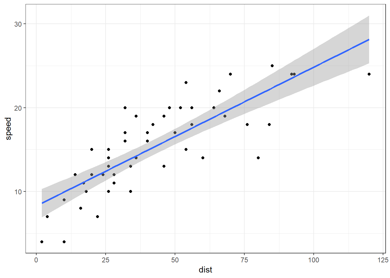
\(~\)
\(~\)
Sob a abordagem bayesiana, a distribuição Normal-Inversa Gama (NIG) é uma priori conjugada para \(\boldsymbol{\theta} = (\boldsymbol{\beta},\sigma^2)\) neste modelo. Assim, \[(\boldsymbol{\beta},\sigma^2) \sim \textit{NIG}(\boldsymbol{\beta}_0, \boldsymbol{V}_0, a_0, b_0)~.\]
Isto é,
\(\boldsymbol{\beta} | \sigma^2 \sim Normal_p\left(\boldsymbol{\beta}_0,\sigma^2\boldsymbol{V}_0\right)~~\); \(~~ \sigma^2 \sim InvGamma\left(a_0,b_0\right)\)
ou, equivalentemente,
\(\boldsymbol{\beta} \sim T_p\left(2a_0; \boldsymbol{\beta}_0,\frac{b_0 \boldsymbol{V}_0}{a_0}\right) ~~\); \(~~ \sigma^2 | \boldsymbol{\beta} \sim InvGamma\left(a_0 + \frac{p}{2},b_0 + \frac{\left(\boldsymbol{\beta}-\boldsymbol{\beta}_0\right)^T \boldsymbol{V}_0^{-1} \left(\boldsymbol{\beta}-\boldsymbol{\beta}_0\right) }{2}\right)~~\),
com \(\boldsymbol{\beta}_0 \in \mathbb{R}^p\), \(\boldsymbol{V}_0\) matriz simétrica positiva definida e \(a_0, b_0 \in \mathbb{R}_+\).
\(~\)
Então: \[(\boldsymbol{\beta},\sigma^2)|\boldsymbol{Z} \sim \textit{NIG}(\boldsymbol{\beta}_1, \boldsymbol{V}_1, a_1, b_1)\]
com \(\boldsymbol{\beta}_1 = \boldsymbol{V}_1\left(\boldsymbol{V}_0^{-1}\boldsymbol{\beta}_0 + \boldsymbol{X}^T\boldsymbol{X} \hat{\boldsymbol{\beta}}\right) ~~\); \(~~ \boldsymbol{V}_1 = \left(\boldsymbol{V}_0^{-1} + \boldsymbol{X}^T\boldsymbol{X}\right)^{-1}~~\); \(a_1 = a_0+\frac{n}{2} ~~\); \(~~ b_1 = b_0 + \frac{\boldsymbol{\beta}_0^T\boldsymbol{V}_0^{-1}\boldsymbol{\beta}_0 + \boldsymbol{Y}^T\boldsymbol{Y} - \boldsymbol{\beta}_1^T\boldsymbol{V}_1^{-1}\boldsymbol{\beta}_1}{2}\).
\(~\)
Observação. Uma das maneiras de representar falta de informação nesse contexto é utilizar a priori de Jeffreys, \(f(\boldsymbol \theta) = \Big|~\mathcal{I}(\boldsymbol \theta)~\Big|^{1/2} \propto 1/\sigma^2\). Nesse caso, distribuição a posteriori é \[(\boldsymbol{\beta},\sigma^2)\Big|\boldsymbol{Z} \sim \textit{NIG}\left(\hat{\boldsymbol{\beta}}, \left(\boldsymbol{X}^T\boldsymbol{X}\right)^{-1}, \dfrac{n-p}{2}, \dfrac{(n-p)s^2}{2}\right)~.\]
\(~\)
\(~\)
Exemplo. Considere que, a priori, \((\boldsymbol{\beta},\sigma^2) \sim \textit{NIG}\left(\boldsymbol{\beta}_0, \boldsymbol{V}_0, a_0, b_0\right)\), com \(~\boldsymbol{\beta}_0 = \left[\begin{array}{c} 0\\0\end{array}\right]~\); \(~\boldsymbol{V}_0 = \left[\begin{array}{cc} 100 & 0\\ 0 & 100\end{array}\right] ~\); \(~a_0 = 3~\); \(~b_0 = 100~\).
A seguir são apresentadas as distribuições marginais dos parâmetros, a distribuição marginal e as regiões HPD bivariadas do parâmetro \(\boldsymbol{\beta}\).
x = cars$dist   # variável resposta
y = cars$speed  # variável explicativa
n = length(x)   # n=50
X = cbind(1,x)  # Matrix de planejamento
p = ncol(X)     # p=2
g = n-p         # gl=48
beta_est = solve(t(X)%*%X)%*%(t(X)%*%y) # (-17.6, 3.9)
sigma_est =
  as.double(t(y-X%*%beta_est)%*%(y-X%*%beta_est)/(n-p)) #236.5
beta0 = c(0,0)                     # média priori betas
V0 = matrix(c(100,0,0,100),ncol=2) # matriz de escala beta
a0 = 3                             # priori sigma
b0 = 100                           # priori sigma
# parâmetros da posteriori
V1 = solve(solve(V0) + t(X)%*%X)
beta1 = V1%*%(solve(V0)%*%beta0 + t(X)%*%X%*%beta_est)
a1 = a0 + n/2
b1 = as.double(b0 + (t(beta0)%*%solve(V0)%*%beta0 + t(y)%*%y - t(beta1)%*%solve(V1)%*%beta1)/2)
V = b1*V1/a1 # Matrix de escala da posteriori marginal de beta

beta1lim=c(beta1[1]-qt(0.9999,2*a1)*sqrt(V[1,1]),beta1[1]+qt(0.9999,2*a1)*sqrt(V[1,1]))
beta2lim=c(beta1[2]-qt(0.9999,2*a1)*sqrt(V[2,2]),beta1[2]+qt(0.9999,2*a1)*sqrt(V[2,2]))
sigma2lim=c(extraDistr::qinvgamma(0.0001,a1,b1),extraDistr::qinvgamma(0.9999,a1,b1))

b1plot <- ggplot(data.frame(x=beta1lim), aes(x=x), colour = "0.Posterior") +
  stat_function(fun = mnormt::dmt,args = list(mean = beta1[1], S = V[1,1], df=2*a1)) +
  theme_bw() + xlab(expression(beta[1])) + ylab("Posterior")
b2plot <- ggplot(data.frame(x=beta2lim), aes(x=x), colour = "0.Posterior") +
  stat_function(fun = mnormt::dmt, args = list(mean = beta1[2], S = V[2,2], df=2*a1)) +
  theme_bw() + xlab(expression(beta[2])) + ylab("Posterior")
s2plot <- ggplot(data.frame(x=sigma2lim),aes(x=x), colour = "0.Posterior")+
  stat_function(fun = extraDistr::dinvgamma, args = list(alpha = a1, beta = b1)) +
  theme_bw() + xlab(expression(sigma^2)) + ylab("Posterior")
ggpubr::ggarrange(b1plot,b2plot,s2plot,ncol=1)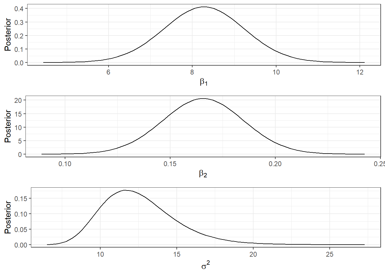
# posteriori marginal bivariada dos betas
posterior <- function(theta0,theta1) { apply(cbind(theta0,theta1),1,function(w){ mnormt::dmt(w, mean=c(beta1), S=V, df=2*a1)  }) }
# Gráfico da posteriori marginal bivariada dos betas
grx <- seq(beta1lim[1], beta1lim[2],length.out=200)
gry <- seq(beta2lim[1], beta2lim[2],length.out=200)
z1 <- outer(grx,gry,posterior)
#persp(grx,gry,z1)
plotly::plot_ly(alpha=0.1) %>%
  plotly::add_surface(x=grx, y=gry, z=t(z1), colorscale = list(c(0,'#BA52ED'), c(1,'#FCB040')), showscale = FALSE)
# Curvas de Probabilidade
l = c(0.1,0.3,0.5,0.8,0.9,0.95,0.99)
z1v = sort(as.vector(z1),decreasing = TRUE)
v1 <- z1v/sum(z1v)
a=0; j=1; l1=NULL
for(i in 1:length(v1)) {
a <- a+v1[i]
if(j<=length(l) & a>l[j]) {
l1 <- c(l1,z1v[i-1])
j <- j+1
}
}
contour(grx,gry,z1,col=colors()[455],main="Regiões HPD para os Betas",xlab=expression(beta[1]),ylab=expression(beta[2]),levels=l1,labels=l)
points(beta1[1],beta1[2],col="darkred",pch=16,cex=0.5)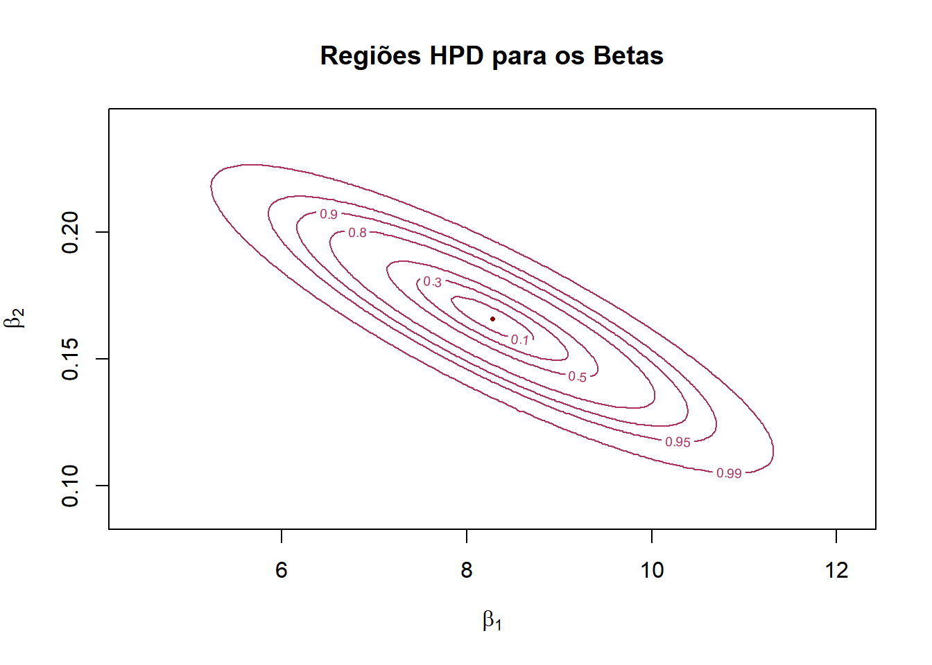
\(~\)
\(~\)
8.2 Laplace’s Demon
LaplacesDemon é uma biblioteca do R que oferece diversos algoritimos implementados de MCMC, permitindo fazer Inferência Bayesiana aproximada. Os algoritimos de MCMC disponíveis são
- Automated Factor Slice Sampler (AFSS)
- Adaptive Directional Metropolis-within-Gibbs (ADMG)
- Adaptive Griddy-Gibbs (AGG)
- Adaptive Hamiltonian Monte Carlo (AHMC)
- Adaptive Metropolis (AM)
- Adaptive Metropolis-within-Gibbs (AMWG)
- Adaptive-Mixture Metropolis (AMM)
- Affine-Invariant Ensemble Sampler (AIES)
- Componentwise Hit-And-Run Metropolis (CHARM)
- Delayed Rejection Adaptive Metropolis (DRAM)
- Delayed Rejection Metropolis (DRM)
- Differential Evolution Markov Chain (DEMC)
- Elliptical Slice Sampler (ESS)
- Gibbs Sampler (Gibbs)
- Griddy-Gibbs (GG)
- Hamiltonian Monte Carlo (HMC)
- Hamiltonian Monte Carlo with Dual-Averaging (HMCDA)
- Hit-And-Run Metropolis (HARM)
- Independence Metropolis (IM)
- Interchain Adaptation (INCA)
- Metropolis-Adjusted Langevin Algorithm (MALA)
- Metropolis-Coupled Markov Chain Monte Carlo (MCMCMC)
- Metropolis-within-Gibbs (MWG)
- Multiple-Try Metropolis (MTM)
- No-U-Turn Sampler (NUTS)
- Oblique Hyperrectangle Slice Sampler (OHSS)
- Preconditioned Crank-Nicolson (pCN)
- Random Dive Metropolis-Hastings (RDMH)
- Random-Walk Metropolis (RWM)
- Reflective Slice Sampler (RSS)
- Refractive Sampler (Refractive)
- Reversible-Jump (RJ)
- Robust Adaptive Metropolis (RAM)
- Sequential Adaptive Metropolis-within-Gibbs (SAMWG)
- Sequential Metropolis-within-Gibbs (SMWG)
- Slice Sampler (Slice)
- Stochastic Gradient Langevin Dynamics (SGLD)
- Tempered Hamiltonian Monte Carlo (THMC)
- t-walk (twalk)
- Univariate Eigenvector Slice Sampler (UESS)
- Updating Sequential Adaptive Metropolis-within-Gibbs (USAMWG)
- Updating Sequential Metropolis-within-Gibbs (USMWG)
\(~\)
Manuais do LaplacesDemon
\(~\)
Voltando ao exemplo de regressão linear:
- Especificação do modelo
require(LaplacesDemon)

parm.names=as.parm.names(list(beta=rep(0,p), sigma2=0))
pos.beta=grep("beta", parm.names)
pos.sigma=grep("sigma2", parm.names)

MyData <- list(J=p, X=X, y=y, mon.names="LP",
  parm.names=parm.names,pos.beta=pos.beta,pos.sigma=pos.sigma)

Model <- function(parm, Data)
{
  ### Parameters
  beta <- parm[Data$pos.beta]
  sigma2 <- interval(parm[Data$pos.sigma], 1e-100, Inf)
  parm[Data$pos.sigma] <- sigma2
  ### Log-Prior
  sigma.prior <- dinvgamma(sigma2, a0, b0, log=TRUE)
  beta.prior <- dmvn(beta, beta0, sigma2*V0, log=TRUE)
  ### Log-Likelihood
  mu <- tcrossprod(Data$X, t(beta))
  LL <- sum(dnormv(Data$y, mu, sigma2, log=TRUE))
  ### Log-Posterior
  LP <- LL + beta.prior + sigma.prior
  Modelout <- list(LP=LP, Dev=-2*LL, Monitor=LP,
                   yhat=rnorm(length(mu), mu, sigma2), parm=parm)
  return(Modelout)
}

Initial.Values <- c(beta_est,sigma_est)

burnin <- 2000
thin <- 3
N=(2000+burnin)*thin- Exemplo 1: Metropolis-within-Gibbs (MWG)
set.seed(666)
Fit1 <- LaplacesDemon(Model, Data=MyData, Initial.Values,
  Covar=NULL, Iterations=N, Status=N/5, Thinning=thin,
  Algorithm="MWG", Specs=NULL)
##
## Laplace's Demon was called on Tue Aug 31 15:30:03 2021
##
## Performing initial checks...
## Algorithm: Metropolis-within-Gibbs
##
## Laplace's Demon is beginning to update...
## Iteration: 2400, Proposal: Componentwise, LP: -146.2
## Iteration: 4800, Proposal: Componentwise, LP: -147.2
## Iteration: 7200, Proposal: Componentwise, LP: -142.7
## Iteration: 9600, Proposal: Componentwise, LP: -143.5
## Iteration: 12000, Proposal: Componentwise, LP: -145.1
##
## Assessing Stationarity
## Assessing Thinning and ESS
## Creating Summaries
## Estimating Log of the Marginal Likelihood
## Creating Output
##
## Laplace's Demon has finished.#names(Fit1)
print(Fit1)## Call:
## LaplacesDemon(Model = Model, Data = MyData, Initial.Values = Initial.Values,
## Covar = NULL, Iterations = N, Status = N/5, Thinning = thin,
## Algorithm = "MWG", Specs = NULL)
##
## Acceptance Rate: 0.35375
## Algorithm: Metropolis-within-Gibbs
## Covariance Matrix: (NOT SHOWN HERE; diagonal shown instead)
## beta[1] beta[2] sigma2
## 1.890044 1.890044 1.890044
##
## Covariance (Diagonal) History: (NOT SHOWN HERE)
## Deviance Information Criterion (DIC):
## All Stationary
## Dbar 258.781 259.440
## pD 4.338 4.237
## DIC 263.119 263.677
## Initial Values:
## [1] 8.2839056 0.1655676 9.9587760
##
## Iterations: 12000
## Log(Marginal Likelihood): -126.8415
## Minutes of run-time: 0.3
## Model: (NOT SHOWN HERE)
## Monitor: (NOT SHOWN HERE)
## Parameters (Number of): 3
## Posterior1: (NOT SHOWN HERE)
## Posterior2: (NOT SHOWN HERE)
## Recommended Burn-In of Thinned Samples: 3200
## Recommended Burn-In of Un-thinned Samples: 9600
## Recommended Thinning: 36
## Specs: (NOT SHOWN HERE)
## Status is displayed every 2400 iterations
## Summary1: (SHOWN BELOW)
## Summary2: (SHOWN BELOW)
## Thinned Samples: 4000
## Thinning: 3
##
##
## Summary of All Samples
## Mean SD MCSE ESS LB
## beta[1] 8.2478022 0.88164035 0.094717679 24.80187 6.6527588
## beta[2] 0.1665176 0.01702535 0.003042654 12.48151 0.1240373
## sigma2 12.5840386 2.48412045 0.125660593 830.27788 8.7682617
## Deviance 258.7813640 2.94533567 0.202218161 136.68013 255.0038715
## LP -143.5465138 1.23958817 0.087107901 109.45812 -146.5361533
## Median UB
## beta[1] 8.2225293 10.1866171
## beta[2] 0.1655676 0.1937371
## sigma2 12.2724404 18.2059419
## Deviance 258.1752506 265.5673438
## LP -143.2451510 -142.1163971
##
##
## Summary of Stationary Samples
## Mean SD MCSE ESS LB
## beta[1] 8.9659139 1.01640981 0.264577460 6.932756 6.5707408
## beta[2] 0.1498047 0.02004864 0.007080864 3.675837 0.1240373
## sigma2 12.4235537 2.25114323 0.223124198 148.522644 8.9164125
## Deviance 259.4399279 2.91101586 0.562252817 35.086016 255.3738557
## LP -143.8933516 1.24169010 0.191055588 27.276956 -146.8229317
## Median UB
## beta[1] 9.0304813 10.6078726
## beta[2] 0.1504279 0.1937371
## sigma2 12.0978375 17.6632608
## Deviance 258.9769661 265.8590137
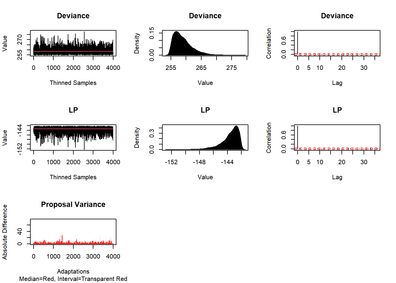
## LP -143.6581852 -142.1644366Post1 <- data.frame(Fit1$Posterior1,Algorithm="1.MWG")
colnames(Post1) <- c("beta1","beta2","sigma2","Algorithm")
#head(Post1)
plot(Fit1, BurnIn=0, MyData, PDF=FALSE, Parms=NULL)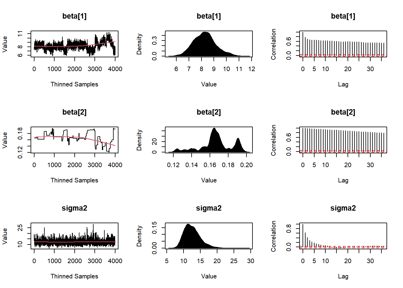
#plot(Fit1, BurnIn=burnin, MyData, PDF=FALSE, Parms=NULL)
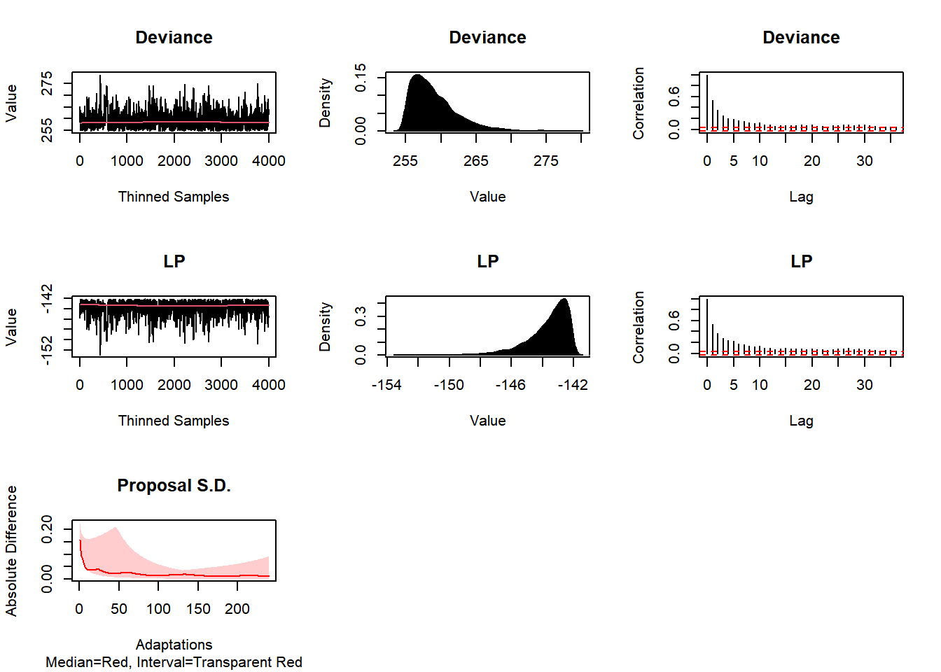
- Exemplo 2: Adaptative Metropolis-within-Gibbs (AMWG)
set.seed(666)
Fit2 <- LaplacesDemon(Model, Data=MyData, Initial.Values,
  Covar=NULL, Iterations=N, Status=N/5, Thinning=thin,
  Algorithm="AMWG", Specs=NULL)
##
## Laplace's Demon was called on Tue Aug 31 15:30:22 2021
##
## Performing initial checks...
## Algorithm: Adaptive Metropolis-within-Gibbs
##
## Laplace's Demon is beginning to update...
## Iteration: 2400, Proposal: Componentwise, LP: -145.3
## Iteration: 4800, Proposal: Componentwise, LP: -143
## Iteration: 7200, Proposal: Componentwise, LP: -144.1
## Iteration: 9600, Proposal: Componentwise, LP: -143.1
## Iteration: 12000, Proposal: Componentwise, LP: -146.2
##
## Assessing Stationarity
## Assessing Thinning and ESS
## Creating Summaries
## Creating Output
##
## Laplace's Demon has finished.#names(Fit2)
#print(Fit2)
Post2 <- data.frame(Fit2$Posterior1,Algorithm="2.AMWG")
colnames(Post2) <- c("beta1","beta2","sigma2","Algorithm")
#head(Post2)
#plot(Fit2, BurnIn=burnin, MyData, PDF=FALSE, Parms=NULL)
plot(Fit2, BurnIn=0, MyData, PDF=FALSE, Parms=NULL)
Post <- rbind(Post1,Post2)
b1plot <- ggplot(Post) +
  stat_function(aes(colour="0.Posterior"), fun = mnormt::dmt,args = list(mean = beta1[1], S = V[1,1], df=2*a1)) +
  geom_density(aes(beta1, colour = Algorithm)) + theme_bw() +
  xlab(expression(beta[1])) + ylab("Posterior") + labs(colour = "Method")
b2plot <- ggplot(Post) +
  stat_function(aes(colour="0.Posterior"), fun = mnormt::dmt, args = list(mean = beta1[2], S = V[2,2], df=2*a1)) +
  geom_density(aes(beta2, colour = Algorithm)) + theme_bw() +
  xlab(expression(beta[2])) + ylab("Posterior") + labs(colour = "Method")
s2plot <- ggplot(Post)+
  stat_function(aes(colour="0.Posterior"), fun = extraDistr::dinvgamma, args = list(alpha = a1, beta = b1)) +
  geom_density(aes(sigma2, colour = Algorithm)) + theme_bw() +
  xlab(expression(sigma^2)) + ylab("Posterior") + labs(colour = "Method")
ggpubr::ggarrange(b1plot,b2plot,s2plot,
                  ncol=1,common.legend=TRUE,legend="bottom")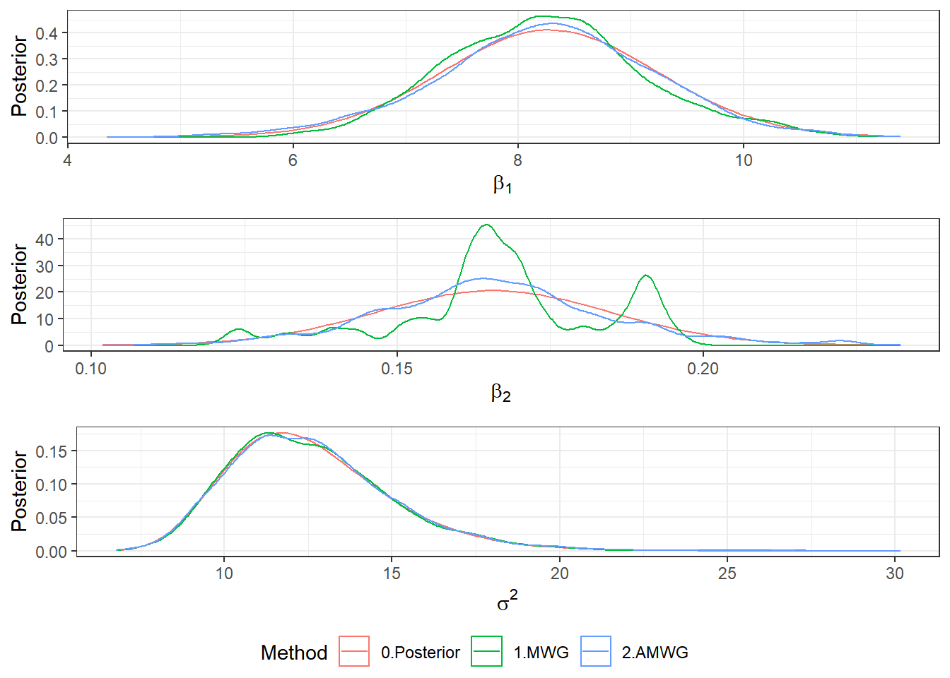
- Exemplo 3: Consort e Automated Factor Slice Sampler (AFSS)
Consort(Fit2)##
## #############################################################
## # Consort with Laplace's Demon #
## #############################################################
## Call:
## LaplacesDemon(Model = Model, Data = MyData, Initial.Values = Initial.Values,
## Covar = NULL, Iterations = N, Status = N/5, Thinning = thin,
## Algorithm = "AMWG", Specs = NULL)
##
## Acceptance Rate: 0.34264
## Algorithm: Adaptive Metropolis-within-Gibbs
## Covariance Matrix: (NOT SHOWN HERE; diagonal shown instead)
## beta[1] beta[2] sigma2
## 1.17679178 0.02838563 9.45831955
##
## Covariance (Diagonal) History: (NOT SHOWN HERE)
## Deviance Information Criterion (DIC):
## All Stationary
## Dbar 258.957 258.957
## pD 4.957 4.957
## DIC 263.915 263.915
## Initial Values:
## [1] 8.2839056 0.1655676 9.9587760
##
## Iterations: 12000
## Log(Marginal Likelihood): NA
## Minutes of run-time: 0.32
## Model: (NOT SHOWN HERE)
## Monitor: (NOT SHOWN HERE)
## Parameters (Number of): 3
## Posterior1: (NOT SHOWN HERE)
## Posterior2: (NOT SHOWN HERE)
## Recommended Burn-In of Thinned Samples: 0
## Recommended Burn-In of Un-thinned Samples: 0
## Recommended Thinning: 105
## Specs: (NOT SHOWN HERE)
## Status is displayed every 2400 iterations
## Summary1: (SHOWN BELOW)
## Summary2: (SHOWN BELOW)
## Thinned Samples: 4000
## Thinning: 3
##
##
## Summary of All Samples
## Mean SD MCSE ESS LB
## beta[1] 8.2386566 0.97788924 0.085914819 151.0105 6.1651888
## beta[2] 0.1661183 0.01903241 0.002099194 209.2080 0.1294318
## sigma2 12.5980978 2.45984860 0.071949821 1784.2000 8.7806779
## Deviance 258.9573762 3.14870026 0.163068368 595.3985 255.1347857
## LP -143.6311506 1.33506450 0.072413145 530.5654 -147.0582460
## Median UB
## beta[1] 8.2641629 10.1040670
## beta[2] 0.1655676 0.2078131
## sigma2 12.3274919 18.1748415
## Deviance 258.2440979 266.8653177
## LP -143.2679823 -142.1324005
##
##
## Summary of Stationary Samples
## Mean SD MCSE ESS LB
## beta[1] 8.2386566 0.97788924 0.085914819 151.0105 6.1651888
## beta[2] 0.1661183 0.01903241 0.002099194 209.2080 0.1294318
## sigma2 12.5980978 2.45984860 0.071949821 1784.2000 8.7806779
## Deviance 258.9573762 3.14870026 0.163068368 595.3985 255.1347857
## LP -143.6311506 1.33506450 0.072413145 530.5654 -147.0582460
## Median UB
## beta[1] 8.2641629 10.1040670
## beta[2] 0.1655676 0.2078131
## sigma2 12.3274919 18.1748415
## Deviance 258.2440979 266.8653177
## LP -143.2679823 -142.1324005
##
## Demonic Suggestion
##
## Due to the combination of the following conditions,
##
## 1. Adaptive Metropolis-within-Gibbs
## 2. The acceptance rate (0.3426389) is within the interval [0.15,0.5].
## 3. At least one target MCSE is >= 6.27% of its marginal posterior
## standard deviation.
## 4. Each target distribution has an effective sample size (ESS)
## of at least 100.
## 5. Each target distribution became stationary by
## 1 iteration.
##
## Quantiles of Absolute Posterior1 Correlation:
## 0% 25% 50% 75% 100%
## 0.02856704 0.03170699 0.85367854 1.00000000 1.00000000
##
## Possibly excessive posterior correlation for a componentwise algorithm.
##
## WARNING: Diminishing adaptation did not occur.
## A new algorithm will be suggested.
##
## Laplace's Demon has not been appeased, and suggests
## copy/pasting the following R code into the R console,
## and running it.
##
## Initial.Values <- as.initial.values(Fit2)
## Fit2 <- LaplacesDemon(Model, Data=MyData, Initial.Values,
## Covar=Fit2$Covar, Iterations=420000, Status=37500, Thinning=105,
## Algorithm="AFSS", Specs=list(A=Inf, B=NULL, m=100,
## n=0, w=1))
##
## Laplace's Demon is finished consorting.Initial.Values <- as.initial.values(Fit2)
set.seed(666)
Fit3 <- LaplacesDemon(Model, Data=MyData, Initial.Values,
Covar=NULL, Iterations=N, Status=N/5, Thinning=thin,
Algorithm="AFSS", Specs=list(A=Inf, B=NULL, m=100,n=0, w=1))##
## Laplace's Demon was called on Tue Aug 31 15:30:50 2021
##
## Performing initial checks...
## Algorithm: Automated Factor Slice Sampler
##
## Laplace's Demon is beginning to update...
##
## Eigendecomposition will occur every 120 iterations.
##
## Iteration: 2400, Proposal: Multivariate, LP: -142.1
## Iteration: 4800, Proposal: Multivariate, LP: -144.2
## Iteration: 7200, Proposal: Multivariate, LP: -145.2
## Iteration: 9600, Proposal: Multivariate, LP: -144.1
## Iteration: 12000, Proposal: Multivariate, LP: -142.5
##
## Assessing Stationarity
## Assessing Thinning and ESS
## Creating Summaries
## Estimating Log of the Marginal Likelihood
## Creating Output
##
## Laplace's Demon has finished.Post3 <- data.frame(Fit3$Posterior1,Algorithm="3.AFSS")
colnames(Post3) <- c("beta1","beta2","sigma2","Algorithm")
plot(Fit3, BurnIn=0, MyData, PDF=FALSE, Parms=NULL)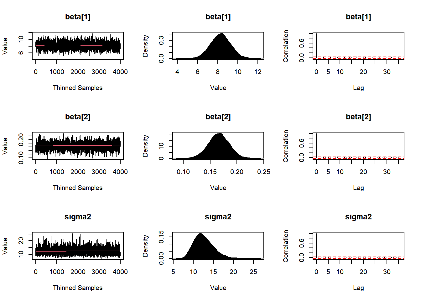
Post <- rbind(Post1,Post2,Post3)
b1plot <- ggplot(Post) +
  stat_function(aes(colour="0.Posterior"), fun = mnormt::dmt,args = list(mean = beta1[1], S = V[1,1], df=2*a1)) +
  geom_density(aes(beta1, colour = Algorithm)) + theme_bw() +
  xlab(expression(beta[1])) + ylab("Posterior") + labs(colour = "Method")
b2plot <- ggplot(Post) +
  stat_function(aes(colour="0.Posterior"), fun = mnormt::dmt, args = list(mean = beta1[2], S = V[2,2], df=2*a1)) +
  geom_density(aes(beta2, colour = Algorithm)) + theme_bw() +
  xlab(expression(beta[2])) + ylab("Posterior") + labs(colour = "Method")
s2plot <- ggplot(Post)+
  stat_function(aes(colour="0.Posterior"), fun = extraDistr::dinvgamma, args = list(alpha = a1, beta = b1)) +
  geom_density(aes(sigma2, colour = Algorithm)) + theme_bw() +
  xlab(expression(sigma^2)) + ylab("Posterior") + labs(colour = "Method")
ggpubr::ggarrange(b1plot,b2plot,s2plot,
                  ncol=1,common.legend=TRUE,legend="bottom")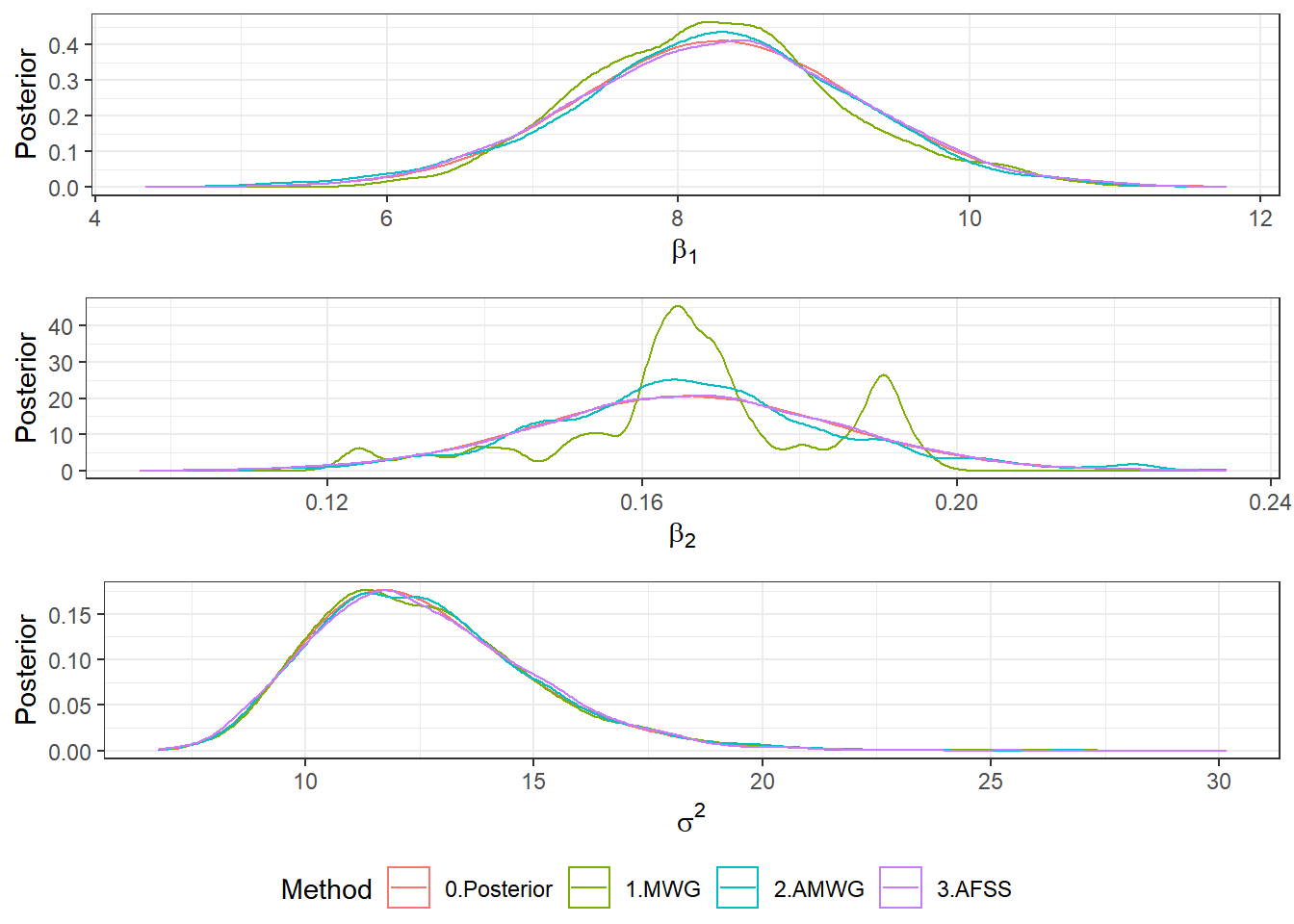
p.interval(Post3$beta2, HPD=TRUE, MM=FALSE, plot=TRUE)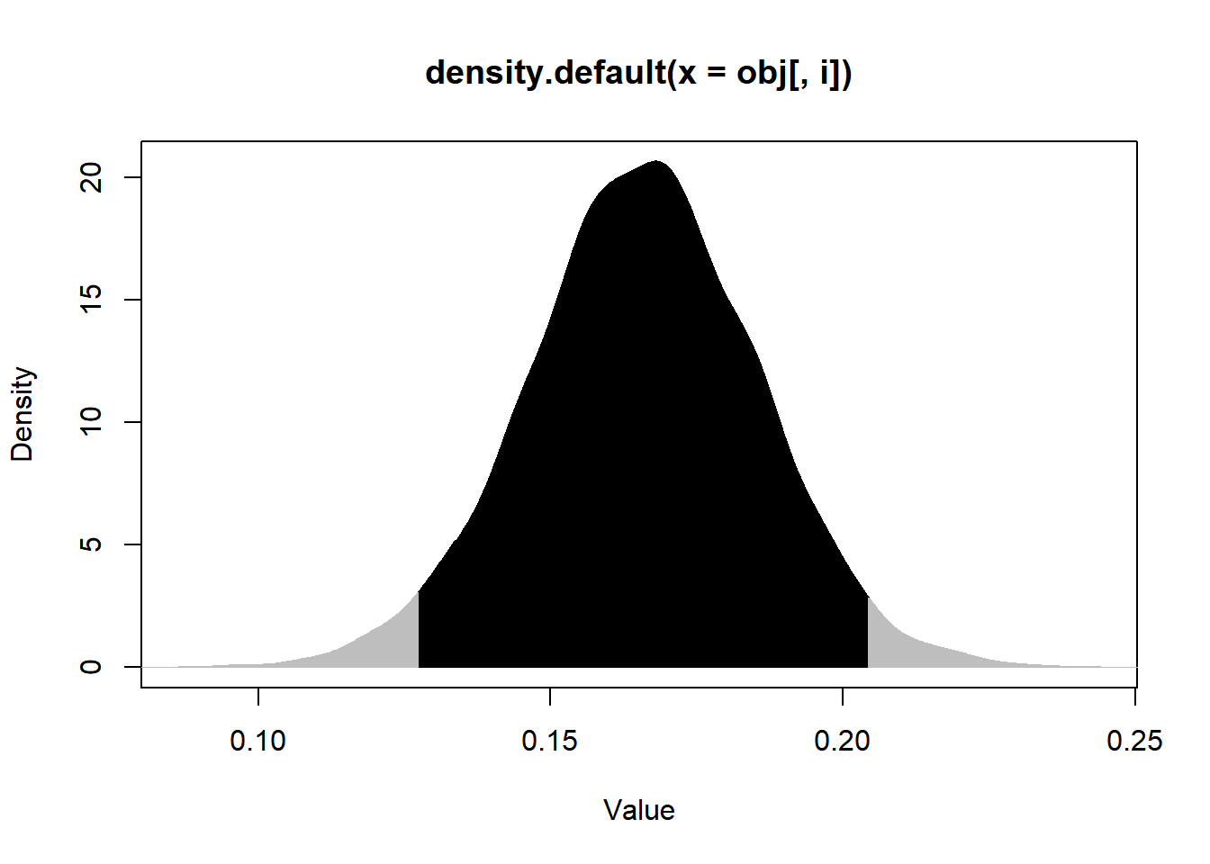
##          Lower     Upper
## [1,] 0.1274793 0.2042041
## attr(,"Probability.Interval")
## [1] 0.95set.seed(666)
S0 <- as.matrix(extraDistr::rinvgamma(N/thin-burnin,a1,b1))
M0 <- apply(S0,1,function(s){mnormt::rmnorm(1,mean=beta1,varcov=s*V1)})
Post0 <- data.frame(t(M0),S0,"0.Posterior")
colnames(Post0) <- c("beta1","beta2","sigma2","Algorithm")
Post = rbind(Post0,Post1,Post2,Post3)
ggplot(Post) + theme_bw() +
geom_point(aes(beta1,beta2,colour=Algorithm), shape=1) +
facet_wrap(Algorithm ~ .) + guides(colour = "none")
8.3 Stan
O Stan é uma plataforma de modelagem estatística de alto desempenho. Em particular, permite fazer inferência bayesiana usando o método de Monte Carlo Hamiltoniano1 (HMC) e a variação No-U-Turn Sampler (NUTS). Esses recursos convergem para distribuições alvo de altas dimensões muito mais rapidamente que métodos mais simples, como o amostrador de Gibbs ou outras variações do método de Metropolis-Hastings. A linguagem utilizada é independente da plataforma e existem bibliotecas para R (rstan) e Python.
Principais manuais do Stan:
\(~\)
Voltando ao Exemplo
library(rstan)
# Parametros do método
Initial.Values <- c(beta_est,sigma_est)
burnin <- 2000
thin <- 3
N=(2000+burnin)*thin
# Conjunto de dados
stan_data <- list(N = n, J = p, y = y, x = X)

# Especificação do modelo
rs_code <- '
  data {
    int<lower=1> N;
    int<lower=1> J;
    matrix[N,J] x;
    vector[N] y;
  }
  parameters {
    vector[J] beta;
    real<lower=0> sigma2;
  }
  model {
    sigma2 ~ inv_gamma(3, 100);
    beta ~ normal(0, sqrt(sigma2*100));
    y ~ normal(x * beta, sqrt(sigma2));
}'

stan_mod <- stan(model_code = rs_code, data = stan_data, init=Initial.Values,
            chains = 1, iter = N, warmup = burnin, thin = thin)
##
## SAMPLING FOR MODEL '6b158d2712aa5479f81bd408884c9453' NOW (CHAIN 1).
## Chain 1:
## Chain 1: Gradient evaluation took 0 seconds
## Chain 1: 1000 transitions using 10 leapfrog steps per transition would take 0 seconds.
## Chain 1: Adjust your expectations accordingly!
## Chain 1:
## Chain 1:
## Chain 1: Iteration: 1 / 12000 [ 0%] (Warmup)
## Chain 1: Iteration: 1200 / 12000 [ 10%] (Warmup)
## Chain 1: Iteration: 2001 / 12000 [ 16%] (Sampling)
## Chain 1: Iteration: 3200 / 12000 [ 26%] (Sampling)
## Chain 1: Iteration: 4400 / 12000 [ 36%] (Sampling)
## Chain 1: Iteration: 5600 / 12000 [ 46%] (Sampling)
## Chain 1: Iteration: 6800 / 12000 [ 56%] (Sampling)
## Chain 1: Iteration: 8000 / 12000 [ 66%] (Sampling)
## Chain 1: Iteration: 9200 / 12000 [ 76%] (Sampling)
## Chain 1: Iteration: 10400 / 12000 [ 86%] (Sampling)
## Chain 1: Iteration: 11600 / 12000 [ 96%] (Sampling)
## Chain 1: Iteration: 12000 / 12000 [100%] (Sampling)
## Chain 1:
## Chain 1: Elapsed Time: 0.282 seconds (Warm-up)
## Chain 1: 1.252 seconds (Sampling)
## Chain 1: 1.534 seconds (Total)
## Chain 1:posterior <- rstan::extract(stan_mod)
Post4 <- data.frame(posterior$beta[,1],posterior$beta[,2],posterior$sigma2,Algorithm="4.RStan")
colnames(Post4) <- c("beta1","beta2","sigma2","Algorithm")
# gráficos posterioris marginais
Post <- rbind(Post3,Post4) %>%
mutate(Algorithm=ifelse(Algorithm=="3.AFSS","1.LaplacesDemons","2.RStan"))
b1plot <- ggplot(Post) +
stat_function(aes(colour="0.Posterior"), fun = mnormt::dmt,args = list(mean = beta1[1], S = V[1,1], df=2*a1)) +
geom_density(aes(beta1, colour = Algorithm)) + theme_bw() +
xlab(expression(beta[1])) + ylab("Posterior") + labs(colour = "Method")
b2plot <- ggplot(Post) +
stat_function(aes(colour="0.Posterior"), fun = mnormt::dmt, args = list(mean = beta1[2], S = V[2,2], df=2*a1)) +
geom_density(aes(beta2, colour = Algorithm)) + theme_bw() +
xlab(expression(beta[2])) + ylab("Posterior") + labs(colour = "Method")
s2plot <- ggplot(Post)+
stat_function(aes(colour="0.Posterior"), fun = extraDistr::dinvgamma, args = list(alpha = a1, beta = b1)) +
geom_density(aes(sigma2, colour = Algorithm)) + theme_bw() +
xlab(expression(sigma^2)) + ylab("Posterior") + labs(colour = "Method")
ggpubr::ggarrange(b1plot,b2plot,s2plot,
ncol=1,common.legend=TRUE,legend="bottom")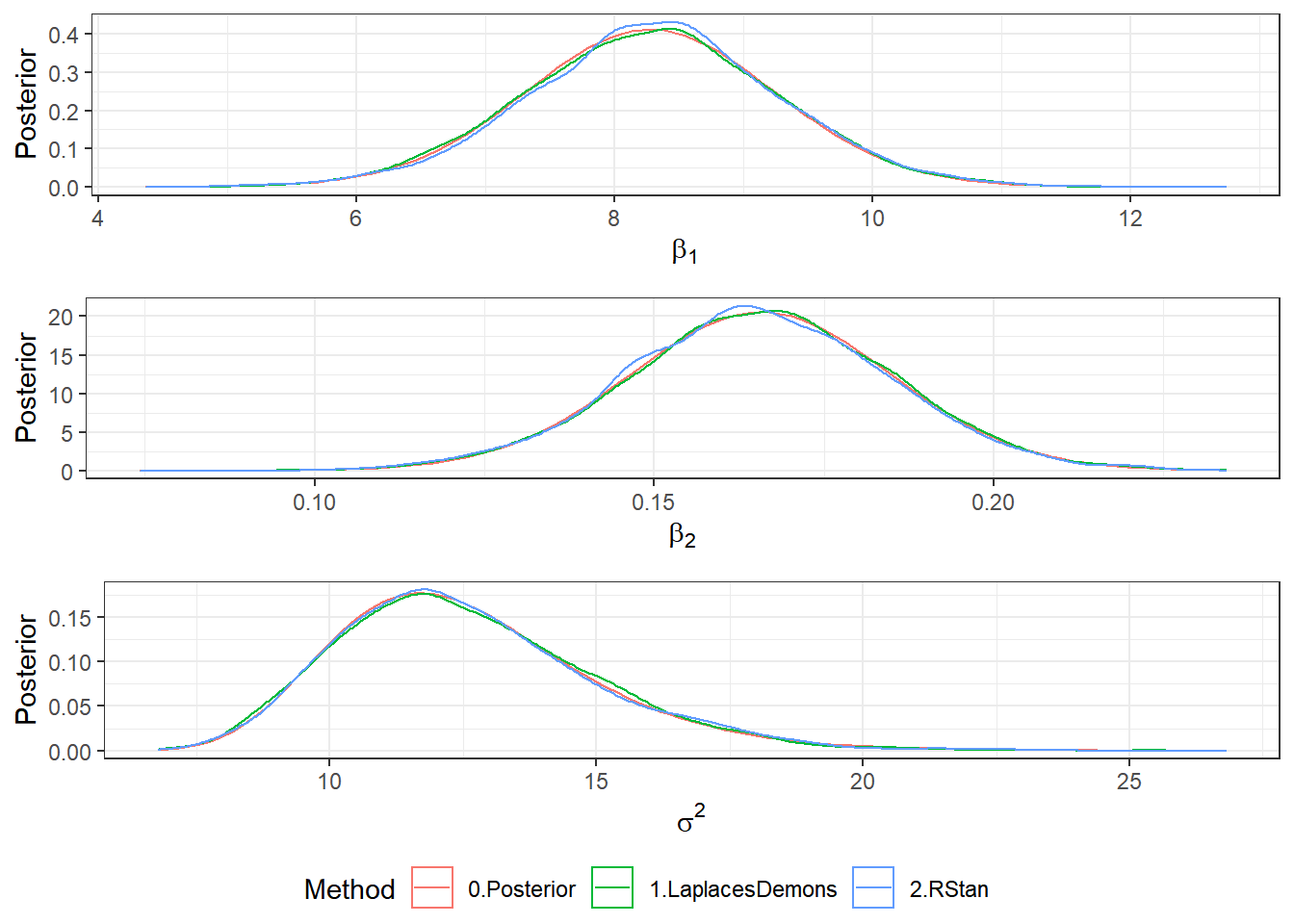
Post = rbind(Post0,Post4) %>%
  mutate(Algorithm=ifelse(Algorithm=="4.RStan","1.RStan","0.Posterior"))
ggplot(Post) + theme_bw() +
  geom_point(aes(beta1,beta2,colour=Algorithm), shape=1) +
  facet_wrap(Algorithm ~ .) + guides(colour = "none")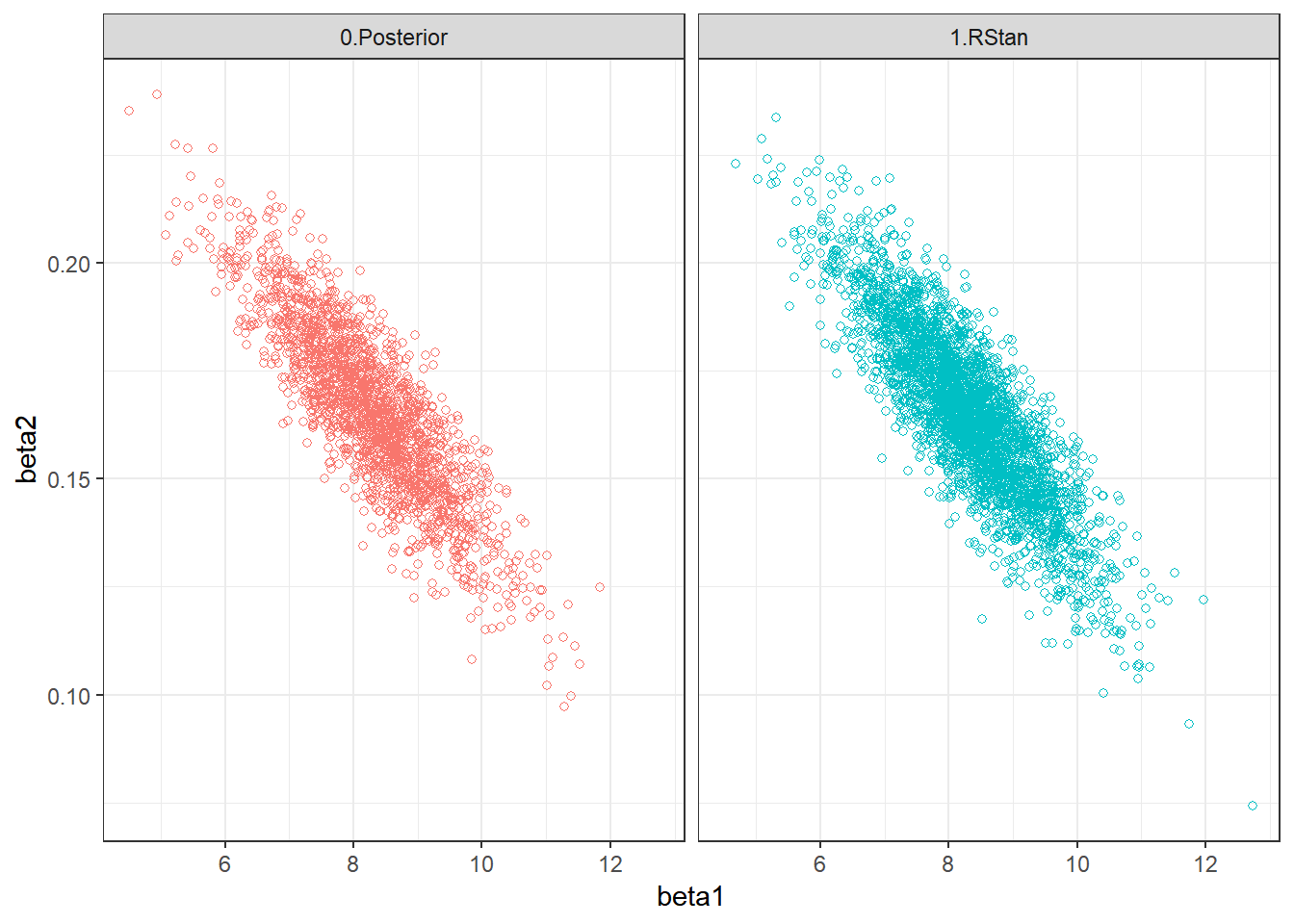
\(~\)
library(ggmcmc)
stan_mod2 <- stan(model_code = rs_code, data = stan_data, init=Initial.Values,
            chains = 2, iter = N, warmup = burnin, thin = thin)
##
## SAMPLING FOR MODEL '6b158d2712aa5479f81bd408884c9453' NOW (CHAIN 1).
## Chain 1:
## Chain 1: Gradient evaluation took 0 seconds
## Chain 1: 1000 transitions using 10 leapfrog steps per transition would take 0 seconds.
## Chain 1: Adjust your expectations accordingly!
## Chain 1:
## Chain 1:
## Chain 1: Iteration: 1 / 12000 [ 0%] (Warmup)
## Chain 1: Iteration: 1200 / 12000 [ 10%] (Warmup)
## Chain 1: Iteration: 2001 / 12000 [ 16%] (Sampling)
## Chain 1: Iteration: 3200 / 12000 [ 26%] (Sampling)
## Chain 1: Iteration: 4400 / 12000 [ 36%] (Sampling)
## Chain 1: Iteration: 5600 / 12000 [ 46%] (Sampling)
## Chain 1: Iteration: 6800 / 12000 [ 56%] (Sampling)
## Chain 1: Iteration: 8000 / 12000 [ 66%] (Sampling)
## Chain 1: Iteration: 9200 / 12000 [ 76%] (Sampling)
## Chain 1: Iteration: 10400 / 12000 [ 86%] (Sampling)
## Chain 1: Iteration: 11600 / 12000 [ 96%] (Sampling)
## Chain 1: Iteration: 12000 / 12000 [100%] (Sampling)
## Chain 1:
## Chain 1: Elapsed Time: 0.376 seconds (Warm-up)
## Chain 1: 0.951 seconds (Sampling)
## Chain 1: 1.327 seconds (Total)
## Chain 1:
##
## SAMPLING FOR MODEL '6b158d2712aa5479f81bd408884c9453' NOW (CHAIN 2).
## Chain 2:
## Chain 2: Gradient evaluation took 0 seconds
## Chain 2: 1000 transitions using 10 leapfrog steps per transition would take 0 seconds.
## Chain 2: Adjust your expectations accordingly!
## Chain 2:
## Chain 2:
## Chain 2: Iteration: 1 / 12000 [ 0%] (Warmup)
## Chain 2: Iteration: 1200 / 12000 [ 10%] (Warmup)
## Chain 2: Iteration: 2001 / 12000 [ 16%] (Sampling)
## Chain 2: Iteration: 3200 / 12000 [ 26%] (Sampling)
## Chain 2: Iteration: 4400 / 12000 [ 36%] (Sampling)
## Chain 2: Iteration: 5600 / 12000 [ 46%] (Sampling)
## Chain 2: Iteration: 6800 / 12000 [ 56%] (Sampling)
## Chain 2: Iteration: 8000 / 12000 [ 66%] (Sampling)
## Chain 2: Iteration: 9200 / 12000 [ 76%] (Sampling)
## Chain 2: Iteration: 10400 / 12000 [ 86%] (Sampling)
## Chain 2: Iteration: 11600 / 12000 [ 96%] (Sampling)
## Chain 2: Iteration: 12000 / 12000 [100%] (Sampling)
## Chain 2:
## Chain 2: Elapsed Time: 0.233 seconds (Warm-up)
## Chain 2: 0.983 seconds (Sampling)
## Chain 2: 1.216 seconds (Total)
## Chain 2:\(~\)
1. Histograma com as cadeias geradas combinadas.
ggs(stan_mod2) %>% ggs_histogram(.) 2. Gráficos das Densidades sobrepostos com cores diferentes por cadeia, permite comparar se as cadeias convergiram para distribuições semelhantes.
ggs(stan_mod2) %>% ggs_density(.)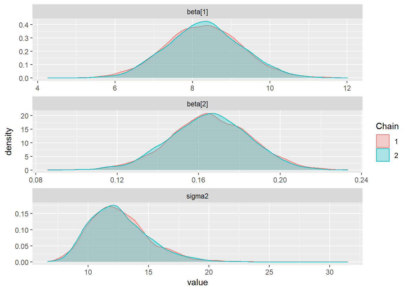 3. Séries Temporais das cadeias geradas. É esperado que as cadeias geradas apresentem distribuições semelhantes em torno de uma mesma média, indicando assim que atingiu-se a “estacionariedade.”
ggs(stan_mod2) %>% ggs_traceplot(.)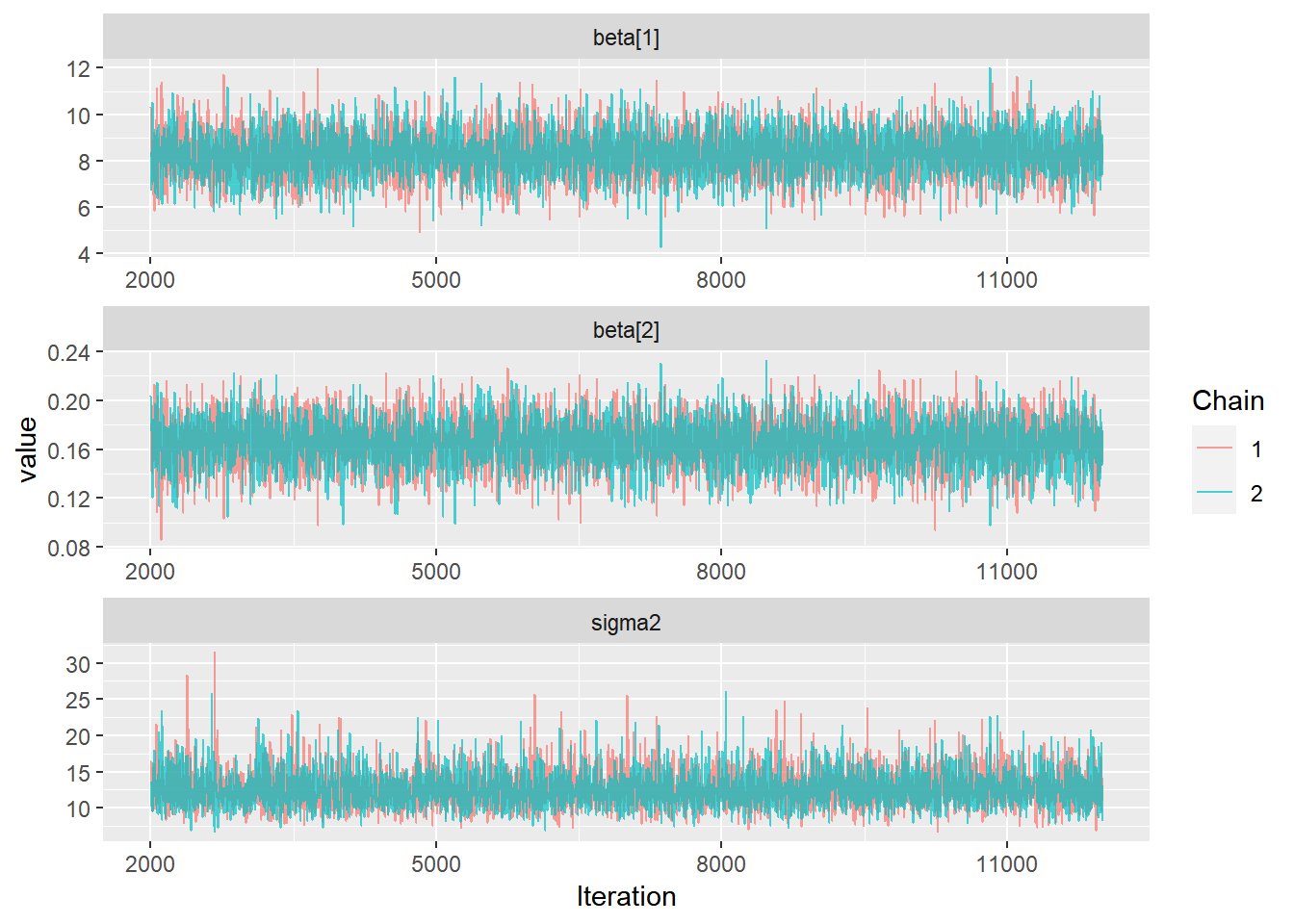 4. Gráfico de Médias Móveis. É esperado que as curvas das médias das cadeias geradas se aproximem rapidamente de um mesmo valor.
ggs(stan_mod2) %>% ggs_running(.)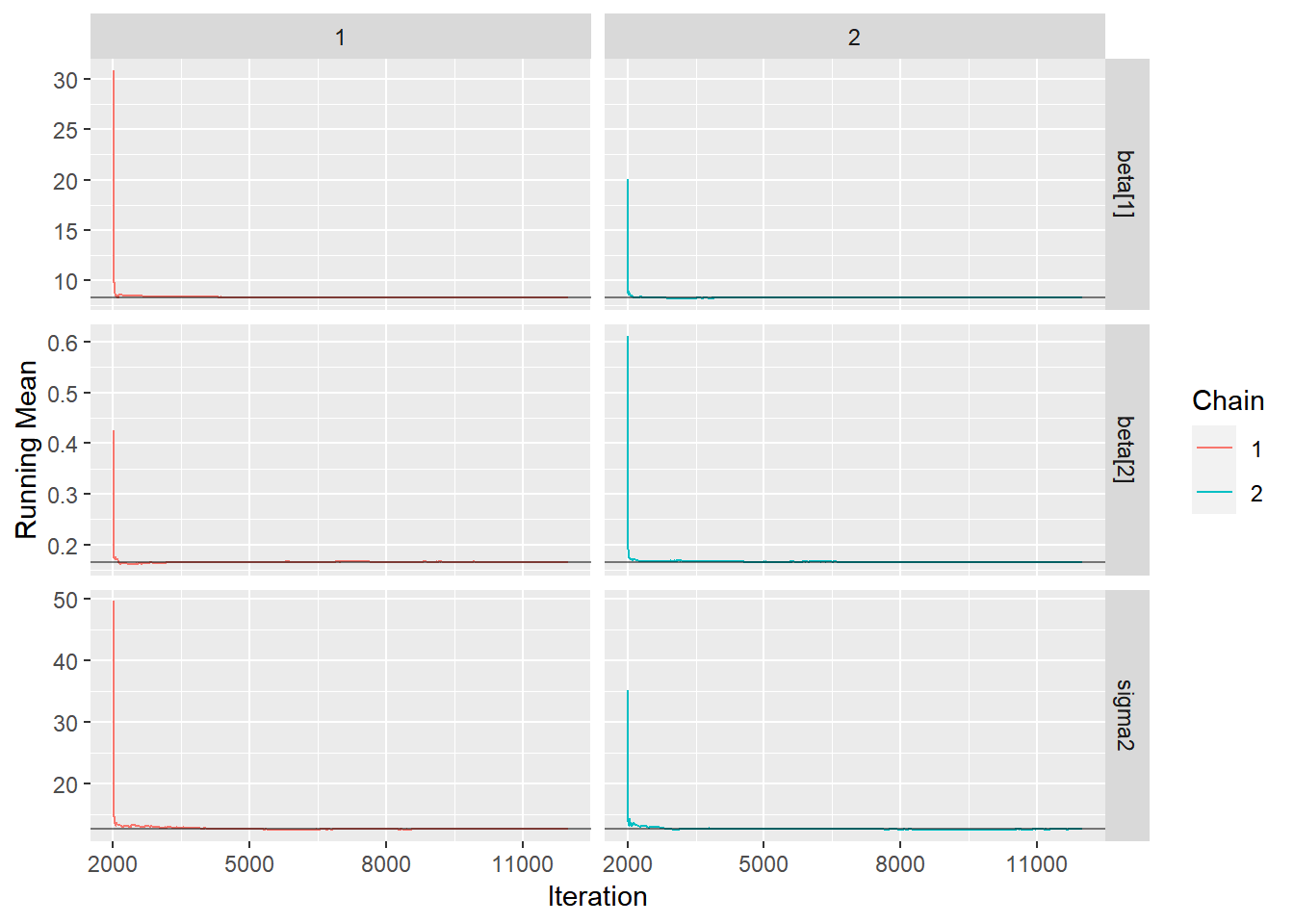
5. Densidades parcial e completa sobrepostas. Compara a última parte da cadeia (por padrão, os últimos 10% dos valores, em verde) com a cadeia inteira (em preto). Idealmente, as partes inicial e final da cadeia devem ser amostradas na mesma distribuição alvo, de modo que as densidades sobrepostas devem ser semelhantes.
ggs(stan_mod2) %>% ggs_compare_partial(.)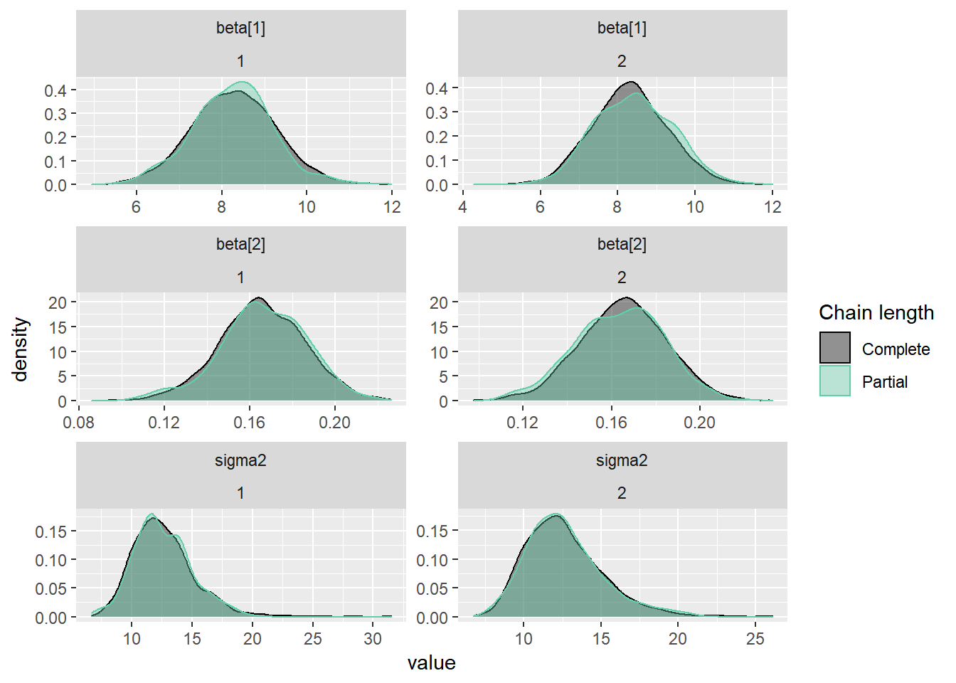
6. Gráfico de Autocorrelação. Espera-se alta correlação apenas no primeiro lag. Quando há um comportamento diferente do esperado, deve-se aumentar o tamanho dos saltos (thin) entre as observações da cadeia gerada que serão consideradas na amostra final.
ggs(stan_mod2) %>% ggs_autocorrelation(.)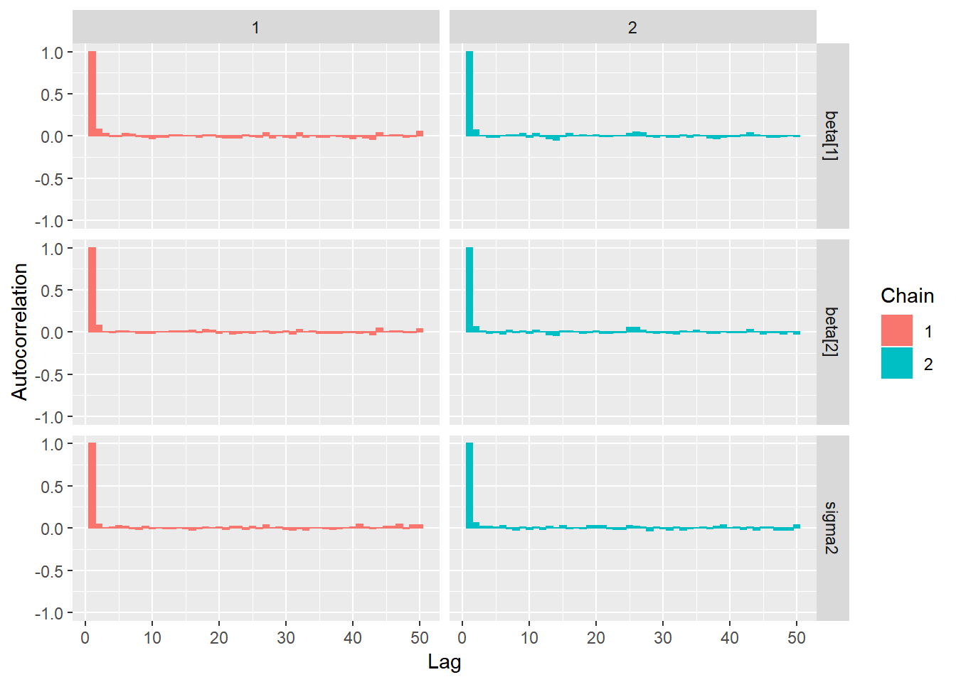
6. Correlação Cruzada. Quando há alta correlação entre os parâmetros é possível que a convergência da cadeia seja mais lenta.
ggs(stan_mod2) %>% ggs_crosscorrelation(.)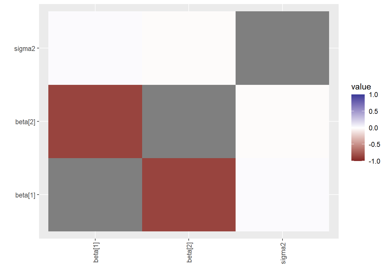
ggs(stan_mod2) %>% ggs_pairs(., lower = list(continuous = "density"))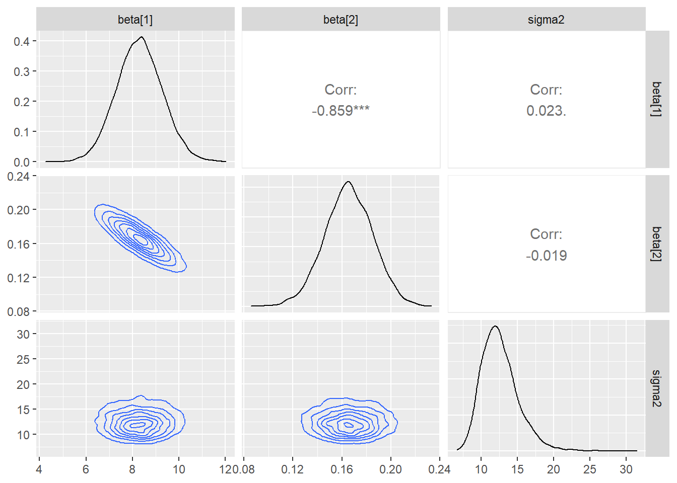
\(~\)
\(~\)
8.4 MLG
O modelos lineares generalizados (MLG) são uma extensão natural dos modelos lineares para casos em que a distribuição da variável resposta não é normal. Como exemplo, vamos considerar o particular caso onde a resposta é binária, conhecido como regressão logística.
Considere \(Y_1,\ldots,Y_n\) condicionalmente independentes tais que \(Y_i|\theta_i \sim \textit{Ber}(\theta_i)\), em que \(\theta_i\) é tal que \(\log\left(\dfrac{\theta_i}{1-\theta_i}\right) = \boldsymbol x_i' \boldsymbol\beta\) ou, em outras palavras, \(\theta_i = \dfrac{1}{1+e^{-\boldsymbol x_i' \boldsymbol\beta}} = \dfrac{e^{\boldsymbol x_i' \boldsymbol\beta}}{1+e^{\boldsymbol x_i' \boldsymbol\beta}}\) com \(\boldsymbol x_i\) as covariáveis da \(i\)-ésima observação e o vetor de parâmetros \(\boldsymbol\beta=(\beta_1,\ldots,\beta_p)\).
\(~\)
Exemplo. Considere as variáveis vs (0 = motor em forma de V, 1 = motor reto) e mpg (milhas/galão(EUA)) do conjunto de dados mtcars do R. Suponha um modelo de regressão logística para a variável resposta vs com a covariável mpg em que, a priori, \(\beta_i \sim \textit{Laplace}(0,b_i)\), \(i=1,2\), independentes. Deste modo, a posteriori é dada por
\(f(\boldsymbol\beta | \boldsymbol{y},\boldsymbol{x})\) \(\propto f(\boldsymbol{y}|\boldsymbol\beta,\boldsymbol{x})f(\boldsymbol\beta)\) \(\propto \displaystyle\prod_{i=1}^{n} \left(\dfrac{1}{1+e^{\boldsymbol x_i' \boldsymbol\beta}}\right)^{y_i}\left(\dfrac{e^{\boldsymbol x_i' \boldsymbol\beta}}{1+e^{\boldsymbol x_i' \boldsymbol\beta}}\right)^{1-y_i} \prod_{j=1}^{p} \dfrac{1}{2b_i} e^{-\frac{|\beta_i|}{b_i}}\).
require(tidyverse)
require(rstan)

dados <- tibble(mtcars)
# mpg:  Miles/(US)gallon ;  vs: Engine(0=V-shaped,1=straight)
dados %>% ggplot(aes(group=as.factor(vs),y=mpg,fill=as.factor(vs))) +
        geom_boxplot() + scale_fill_discrete(name="vs") + theme_bw()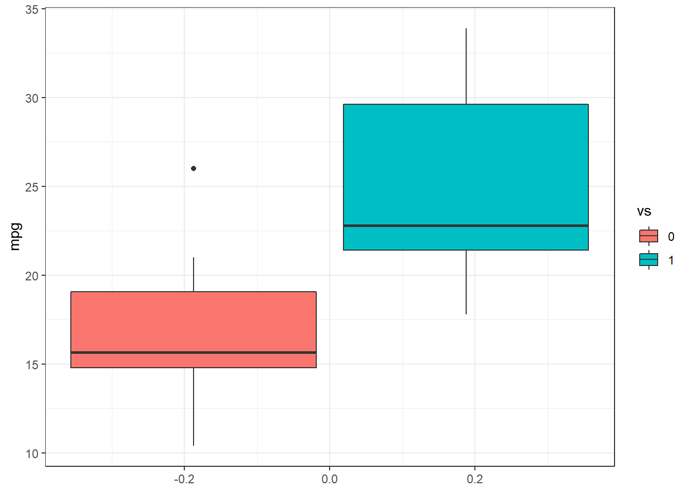
y <- dados %>% select(vs) %>% pull()
x <- dados %>% select(mpg) %>% pull()
n <- length(y)
X <- as.matrix(cbind(1,x))
p <- ncol(X)

# summary(glm(y~x,family=binomial))

stan_data <- list(N = n, J = p, y = y, x = X)

rs_code <- '
  data {
    int<lower=1> N;
    int<lower=1> J;
    int<lower=0,upper=1> y[N];
    matrix[N,J] x;
  }
  parameters {
    vector[J] beta;
  }
  model {
    beta ~ double_exponential(0, 100);
    y ~ bernoulli_logit(x * beta);
  }'

N=2000
thin=10
burnin=1000
set.seed(666)

stan_log <- stan(model_code = rs_code, data = stan_data, init = c(0,0),
  chains = 2, iter = N*thin, warmup = burnin, thin = thin)
##
## SAMPLING FOR MODEL '6525180a46ff3a51f06bbb110d962a1c' NOW (CHAIN 1).
## Chain 1:
## Chain 1: Gradient evaluation took 0 seconds
## Chain 1: 1000 transitions using 10 leapfrog steps per transition would take 0 seconds.
## Chain 1: Adjust your expectations accordingly!
## Chain 1:
## Chain 1:
## Chain 1: Iteration: 1 / 20000 [ 0%] (Warmup)
## Chain 1: Iteration: 1001 / 20000 [ 5%] (Sampling)
## Chain 1: Iteration: 3000 / 20000 [ 15%] (Sampling)
## Chain 1: Iteration: 5000 / 20000 [ 25%] (Sampling)
## Chain 1: Iteration: 7000 / 20000 [ 35%] (Sampling)
## Chain 1: Iteration: 9000 / 20000 [ 45%] (Sampling)
## Chain 1: Iteration: 11000 / 20000 [ 55%] (Sampling)
## Chain 1: Iteration: 13000 / 20000 [ 65%] (Sampling)
## Chain 1: Iteration: 15000 / 20000 [ 75%] (Sampling)
## Chain 1: Iteration: 17000 / 20000 [ 85%] (Sampling)
## Chain 1: Iteration: 19000 / 20000 [ 95%] (Sampling)
## Chain 1: Iteration: 20000 / 20000 [100%] (Sampling)
## Chain 1:
## Chain 1: Elapsed Time: 0.338 seconds (Warm-up)
## Chain 1: 3.141 seconds (Sampling)
## Chain 1: 3.479 seconds (Total)
## Chain 1:
##
## SAMPLING FOR MODEL '6525180a46ff3a51f06bbb110d962a1c' NOW (CHAIN 2).
## Chain 2:
## Chain 2: Gradient evaluation took 0 seconds
## Chain 2: 1000 transitions using 10 leapfrog steps per transition would take 0 seconds.
## Chain 2: Adjust your expectations accordingly!
## Chain 2:
## Chain 2:
## Chain 2: Iteration: 1 / 20000 [ 0%] (Warmup)
## Chain 2: Iteration: 1001 / 20000 [ 5%] (Sampling)
## Chain 2: Iteration: 3000 / 20000 [ 15%] (Sampling)
## Chain 2: Iteration: 5000 / 20000 [ 25%] (Sampling)
## Chain 2: Iteration: 7000 / 20000 [ 35%] (Sampling)
## Chain 2: Iteration: 9000 / 20000 [ 45%] (Sampling)
## Chain 2: Iteration: 11000 / 20000 [ 55%] (Sampling)
## Chain 2: Iteration: 13000 / 20000 [ 65%] (Sampling)
## Chain 2: Iteration: 15000 / 20000 [ 75%] (Sampling)
## Chain 2: Iteration: 17000 / 20000 [ 85%] (Sampling)
## Chain 2: Iteration: 19000 / 20000 [ 95%] (Sampling)
## Chain 2: Iteration: 20000 / 20000 [100%] (Sampling)
## Chain 2:
## Chain 2: Elapsed Time: 0.194 seconds (Warm-up)
## Chain 2: 3.544 seconds (Sampling)
## Chain 2: 3.738 seconds (Total)
## Chain 2:print(stan_log)## Inference for Stan model: 6525180a46ff3a51f06bbb110d962a1c.
## 2 chains, each with iter=20000; warmup=1000; thin=10;
## post-warmup draws per chain=1900, total post-warmup draws=3800.
##
## mean se_mean sd 2.5% 25% 50% 75% 97.5% n_eff Rhat
## beta[1] -10.25 0.06 3.50 -18.27 -12.30 -9.91 -7.76 -4.52 3629 1
## beta[2] 0.50 0.00 0.17 0.21 0.38 0.49 0.60 0.89 3628 1
## lp__ -13.90 0.02 1.02 -16.61 -14.29 -13.61 -13.17 -12.89 3513 1
##
## Samples were drawn using NUTS(diag_e) at Tue Aug 31 15:35:24 2021.
## For each parameter, n_eff is a crude measure of effective sample size,
## and Rhat is the potential scale reduction factor on split chains (at
## convergence, Rhat=1).require(bayesplot)
post_log <- rstan::extract(stan_log, inc_warmup = TRUE, permuted = FALSE)
color_scheme_set("mix-brightblue-gray")
mcmc_trace(post_log, pars = c("beta[1]", "beta[2]"), n_warmup = 0,
facet_args = list(nrow = 2, labeller = label_parsed))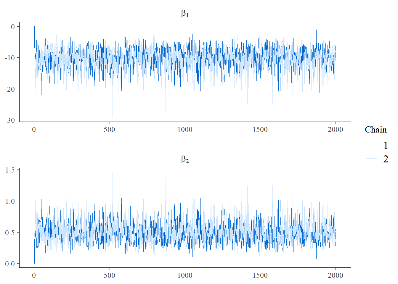
mcmc_acf(post_log, pars = c("beta[1]", "beta[2]"))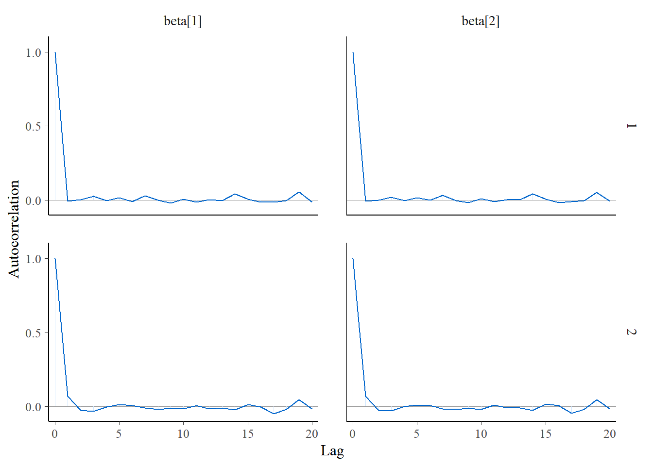
#mcmc_areas(post_log,pars = c("beta[1]", "beta[2]"),prob=0.9)

ggpubr::ggarrange(
  mcmc_areas(post_log,pars = c("beta[1]"),prob=0.9),
  mcmc_areas(post_log,pars = c("beta[2]"),prob=0.9),ncol=1)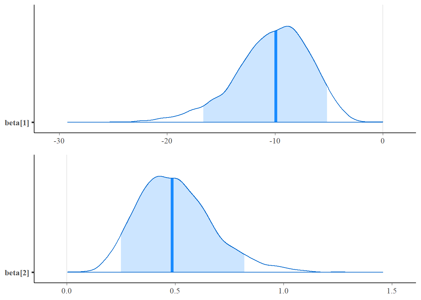
require(ggmcmc)
#ggs(stan_log) %>% ggmcmc(., file = "ggmcmc_log.html")
ggs(stan_log) %>% ggs_pairs(., lower = list(continuous = "density"))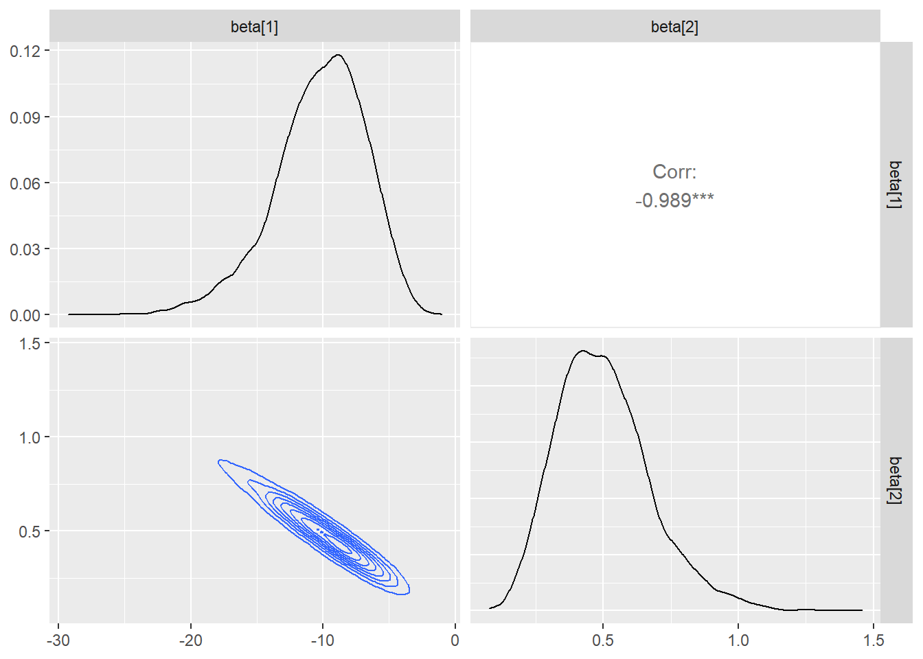
\(~\)
ggs(stan_log)## # A tibble: 7,600 x 4
## Iteration Chain Parameter value
## <dbl> <int> <fct> <dbl>
## 1 1 1 beta[1] -13.5
## 2 2 1 beta[1] -18.3
## 3 3 1 beta[1] -6.63
## 4 4 1 beta[1] -5.45
## 5 5 1 beta[1] -11.7
## 6 6 1 beta[1] -9.19
## 7 7 1 beta[1] -8.40
## 8 8 1 beta[1] -13.9
## 9 9 1 beta[1] -13.6
## 10 10 1 beta[1] -16.5
## # ... with 7,590 more rowslpostlog = Vectorize(function(beta1,beta2){
extraDistr::dlaplace(beta1,mu=0,sigma=100,log=TRUE)+
extraDistr::dlaplace(beta2,mu=0,sigma=100,log=TRUE)+
sum(dbinom(y,1,1/(1+exp(-beta1-beta2*x)),log=TRUE))
})
beta1log=ggs(stan_log) %>% filter(Parameter=="beta[1]") %>% pull()
beta2log=ggs(stan_log) %>% filter(Parameter=="beta[2]") %>% pull()
lpostlog_stan=apply(cbind(beta1log,beta2log),1,
function(t){lpostlog(t[1],t[2])})
gama = c(0.1,0.2,0.3,0.4,0.5,0.6,0.7,0.8,0.9,0.95,0.99)
cortelog = exp(quantile(lpostlog_stan,1-gama))
plot_log = tibble(b1=rep(seq(-24,0,length.out=500),500),
b2=rep(seq(0,1.2,length.out=500),each=500)) %>%
mutate(post=exp(lpostlog(b1,b2)))
plot_log %>%
ggplot(aes(x=b1, y=b2, z=post)) + theme_minimal() +
#geom_contour_filled()+
geom_raster(aes(fill = post)) +
scale_fill_distiller(palette = "Spectral", direction = -1) +
geom_contour(breaks=cortelog, colour="darkblue") +
geom_contour(breaks=cortelog[gama==0.95],colour="red",size=1.5)+
xlab(expression(beta[1])) + ylab(expression(beta[2])) +
theme(legend.position = "none")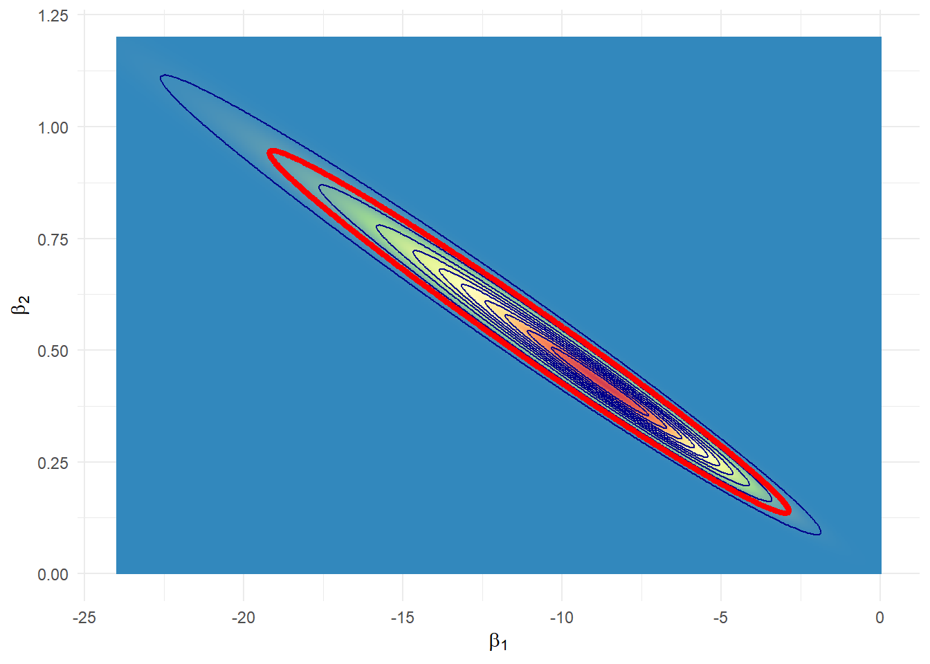
# H: beta_2==0
lpostlog_H = function(beta1){lpostlog(beta1,0)}
suplog_H = optimize(f=lpostlog_H,interval=c(-100,100),maximum=TRUE)$objective
ev_logH = mean(I(lpostlog_stan<suplog_H))
O e-value para testar \(H_0: \beta_2=0\) é 0.
\(~\)
Existe uma biblioteca para modelos lineares bayesianos usando o Stan chamada
rstanarm. Nesta biblioteca, a funçãostan_glmpode ser utilizada para o ajuste de MLGs sob o ponto de vista bayesiano.
\(~\)
\(~\)
8.5 Modelos Dinâmicos
A Biblioteca walker para do R que usa o RStan para fazer inferência bayesiana em modelos lineares com coeficientes variando no tempo (modelos dinâmicos).
Modelo de Regressão Dinâmico Bayesiano
\[y_t = \boldsymbol x_t~\boldsymbol\beta_t + \epsilon_t ~,~~ \epsilon_t \sim \textit{Normal}(0,\sigma_y^2)\] \[\boldsymbol\beta_{t+1} = \boldsymbol\beta_t + \boldsymbol\eta_t ~,~~ \boldsymbol\eta_t \sim \textit{Normal}_k(0,D)\]
onde
\(y_t\): variável resposta no instante \(t\);
\(\boldsymbol x_t\): vetor com \(k\) variáveis preditoras no instante \(t\);
\(\epsilon_t\) e \(\boldsymbol\eta_t\): ruídos brancos;
\(\boldsymbol\beta_t\): vetor dos \(k\) coeficientes de regressão no instante \(t\);
\(D=\textit{diag}({\sigma}_{\eta_i})\);
\(\boldsymbol\sigma=\left(\sigma_y,{\sigma}_{\eta_1},\ldots,{\sigma}_{\eta_k}\right)\): vetor de parâmetros de variância.
As distribuição a piori são dadas por \[\beta_1 \sim \textit{Normal}(m_\beta,{s}_\beta^2)\] \[\sigma_i^2 \sim \textit{Gama}({a}_{\sigma_i},{b}_{\sigma_i})\]
- Sobre a biblioteca
walker:
\(~\)
8.5.1 Dados de Amoxicilina (fonte: CEA)
Dados mensais de venda de Amoxicilina e resistência da bacteria E. coli no período de 01/2008 à 12/2016.
A venda de Amoxicilina foi avaliada pela média mensal das doses diárias definidas por 1000 habitantes-dia (DDD/1000hab/dia), que indica a quantidade média de determinado antibiótico que uma dada população consome diariamente (IMS Health Brazil/Pfizer).
Para avaliar a resistência da bactéria E. coli à Amoxicilina foram utilizados dados obtidos a partir de amostras da rede de apoio do laboratório DASA, que atende principalmente a rede privada de assistência à saúde mas também inclui hospitais que atendem pacientes pelo Sistema Único de Saúde (SUS). Foram incluídas amostras resultantes de exames de sangue e urina positivas, avaliando a proporção de cepas isoladas resistentes à amoxicilina.
Objetivo. Avaliar o impacto da regulamentação RDC 44 da ANVISA que obriga a retenção da prescrição médica para a venda de antimicrobianos, implementada em 26 de Outubro de 2010.
library(lubridate)
dados = read_csv("./data/Amoxicillin.csv") %>%
  select(Período=Periodo,Vendas=DDD1000hab_dia,Resistência=Resistencia_Amoxicilina.Clavulanato.k)
dados$Vendas[61:62]=mean(c(2.073005,2.173923))
mV=mean(dados$Vendas); sdV=sd(dados$Vendas)
mR=mean(dados$Resistência); sdR=sd(dados$Resistência)
Tr <- sdV/sdR # var. aux. para transformação dos eixos
dados %>% ggplot(aes(x=Período)) + theme_bw() +
  geom_line(aes(y=Vendas,colour="Vendas"),lwd=1) + theme(legend.position="bottom") +
  geom_line(aes(x=Período,y=((Resistência-mR)*Tr+mV),colour="Resistência"),lwd=1)+
  labs(y="Vendas de Amoxicilina (DDD/1000 hab./dia)",colour="") +
  scale_y_continuous(sec.axis = sec_axis(~./Tr+(mR-mV/Tr), name = "Prop. de Amostras de E.Colli Resistentes"))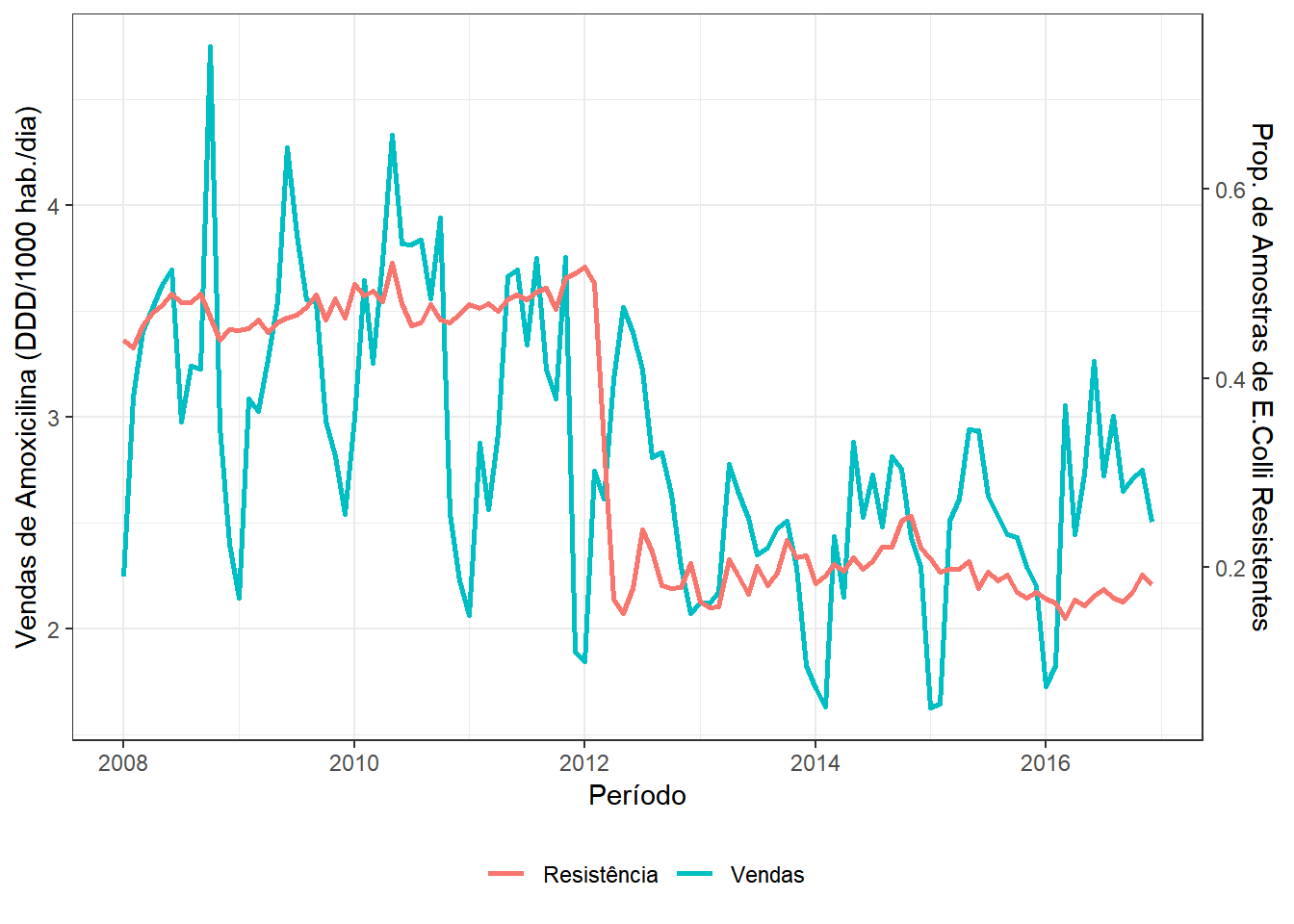
Para verificar se o efeito da venda de antimicrobianos influencia na resistência bacteriana e identificar possíveis mudanças após a implementação da lei, foi considerado um modelo de regressão dinâmico bayesiano, descrito a seguir.
\[(Y_t-\bar{Y_0}) = \beta_t (X_t-\bar{X_0}) + \epsilon_t ~,~~ \epsilon_t \sim Normal(0,\sigma_y^2)\]
\[\beta_{t+1} = \beta_t + W_t ~,~~ W_t \sim Normal(0,\sigma_r^2)\]
\[\sigma_y^2 \sim Gama(2,0.0001)\]
\[\beta_t \sim Normal(0,100)\]
\[\sigma_r^2 \sim Gama(2,0.0001)\]
* \(Y_t\): proporção de testes de resistência positiva do microbiano E. coli no instante \(t\);
* \(X_t\): quantidade de doses consumidas de Amoxicilina (DDD/1000hab/dia) no instante \(t\);
* \(\beta_t\): parâmetro que representa o efeito da venda do antimicrobiano na resistência bacteriana no instante \(t\);
* \(\epsilon_t\) e \(W_t\): ruídos brancos.
require(walker)
set.seed(666)
# resistência média e venda média do período anterior a RDC 44
mAntes = dados %>% filter(year(Período)<2011) %>%
        summarise(mean(Vendas),mean(Resistência)) %>% t()
fit1 <- dados %>%
  mutate(Vendas=Vendas-mAntes[1],Resistência=Resistência-mAntes[2]) %>%
  walker(data=., formula = Resistência ~ -1+rw1(~ -1+Vendas,beta=c(0,100),
    sigma=c(2,0.0001)),sigma_y_prior = c(2,0.0001), chain=2)
##
## SAMPLING FOR MODEL 'walker_lm' NOW (CHAIN 1).
## Chain 1:
## Chain 1: Gradient evaluation took 0.002 seconds
## Chain 1: 1000 transitions using 10 leapfrog steps per transition would take 20 seconds.
## Chain 1: Adjust your expectations accordingly!
## Chain 1:
## Chain 1:
## Chain 1: Iteration: 1 / 2000 [ 0%] (Warmup)
## Chain 1: Iteration: 200 / 2000 [ 10%] (Warmup)
## Chain 1: Iteration: 400 / 2000 [ 20%] (Warmup)
## Chain 1: Iteration: 600 / 2000 [ 30%] (Warmup)
## Chain 1: Iteration: 800 / 2000 [ 40%] (Warmup)
## Chain 1: Iteration: 1000 / 2000 [ 50%] (Warmup)
## Chain 1: Iteration: 1001 / 2000 [ 50%] (Sampling)
## Chain 1: Iteration: 1200 / 2000 [ 60%] (Sampling)
## Chain 1: Iteration: 1400 / 2000 [ 70%] (Sampling)
## Chain 1: Iteration: 1600 / 2000 [ 80%] (Sampling)
## Chain 1: Iteration: 1800 / 2000 [ 90%] (Sampling)
## Chain 1: Iteration: 2000 / 2000 [100%] (Sampling)
## Chain 1:
## Chain 1: Elapsed Time: 6.336 seconds (Warm-up)
## Chain 1: 6.528 seconds (Sampling)
## Chain 1: 12.864 seconds (Total)
## Chain 1:
##
## SAMPLING FOR MODEL 'walker_lm' NOW (CHAIN 2).
## Chain 2:
## Chain 2: Gradient evaluation took 0.001 seconds
## Chain 2: 1000 transitions using 10 leapfrog steps per transition would take 10 seconds.
## Chain 2: Adjust your expectations accordingly!
## Chain 2:
## Chain 2:
## Chain 2: Iteration: 1 / 2000 [ 0%] (Warmup)
## Chain 2: Iteration: 200 / 2000 [ 10%] (Warmup)
## Chain 2: Iteration: 400 / 2000 [ 20%] (Warmup)
## Chain 2: Iteration: 600 / 2000 [ 30%] (Warmup)
## Chain 2: Iteration: 800 / 2000 [ 40%] (Warmup)
## Chain 2: Iteration: 1000 / 2000 [ 50%] (Warmup)
## Chain 2: Iteration: 1001 / 2000 [ 50%] (Sampling)
## Chain 2: Iteration: 1200 / 2000 [ 60%] (Sampling)
## Chain 2: Iteration: 1400 / 2000 [ 70%] (Sampling)
## Chain 2: Iteration: 1600 / 2000 [ 80%] (Sampling)
## Chain 2: Iteration: 1800 / 2000 [ 90%] (Sampling)
## Chain 2: Iteration: 2000 / 2000 [100%] (Sampling)
## Chain 2:
## Chain 2: Elapsed Time: 6.799 seconds (Warm-up)
## Chain 2: 7.36 seconds (Sampling)
## Chain 2: 14.159 seconds (Total)
## Chain 2: #Default: chain=4, iter=2000, warmup=1000, thin=1
ggpubr::ggarrange(
mcmc_areas(as.matrix(fit1$stanfit),regex_pars = c("sigma_rw1"),prob=0.9),
mcmc_areas(as.matrix(fit1$stanfit),regex_pars = c("sigma_y"),prob=0.9),
ncol=1)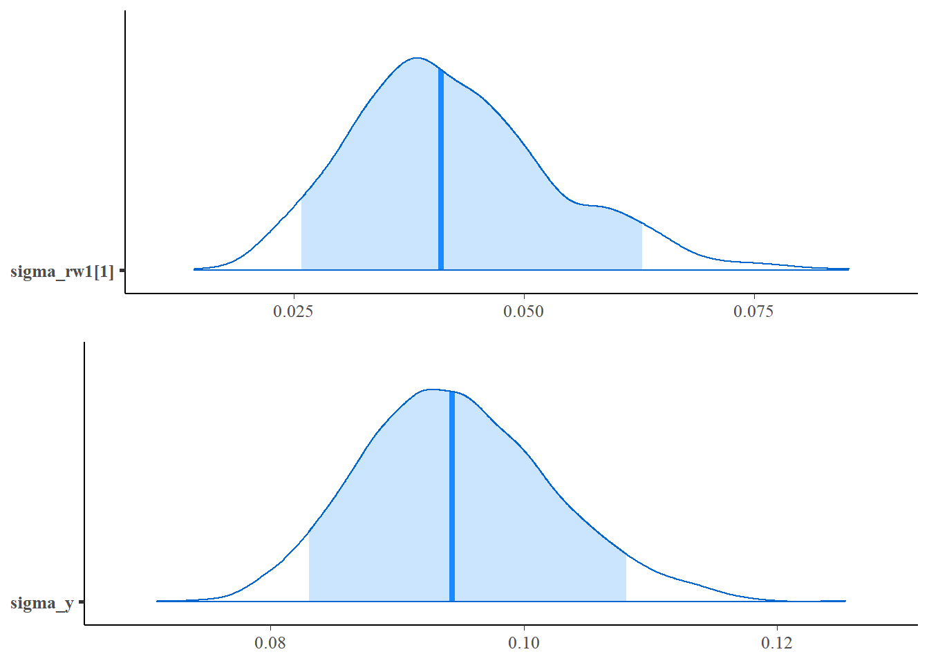
plot_coefs(fit1, scales = "free", alpha=0.8) + theme_bw() +
  scale_x_continuous(breaks=seq(1,length(dados$Período)+1,12),labels=c(unique(year(dados$Período)),2017))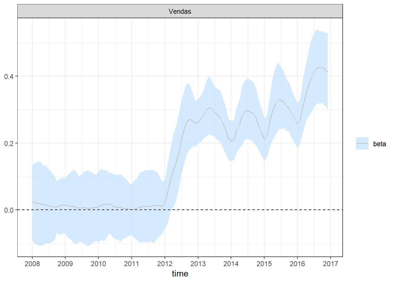
pp_check(fit1, alpha=0.8) + theme_bw() +
  scale_x_continuous(breaks=seq(1,length(dados$Período)+1,12),labels=c(unique(year(dados$Período)),2017))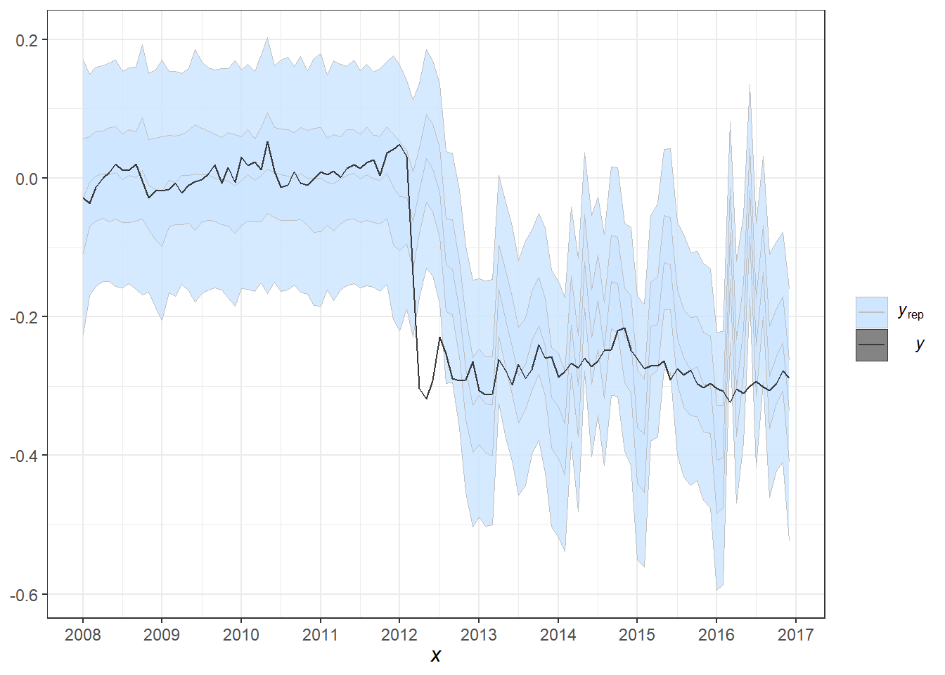
set.seed(666)
new_data <- data.frame(Vendas=seq(dados$Vendas[108]-mAntes[1],-0.2,length.out=12)+c(0,rnorm(11,0,0.08)))
pred1 <- predict(fit1, new_data)
plot_predict(pred1, alpha=0.8) +
  scale_x_continuous(breaks=seq(1,length(dados$Período)+1,12),labels=c(unique(year(dados$Período)),2017))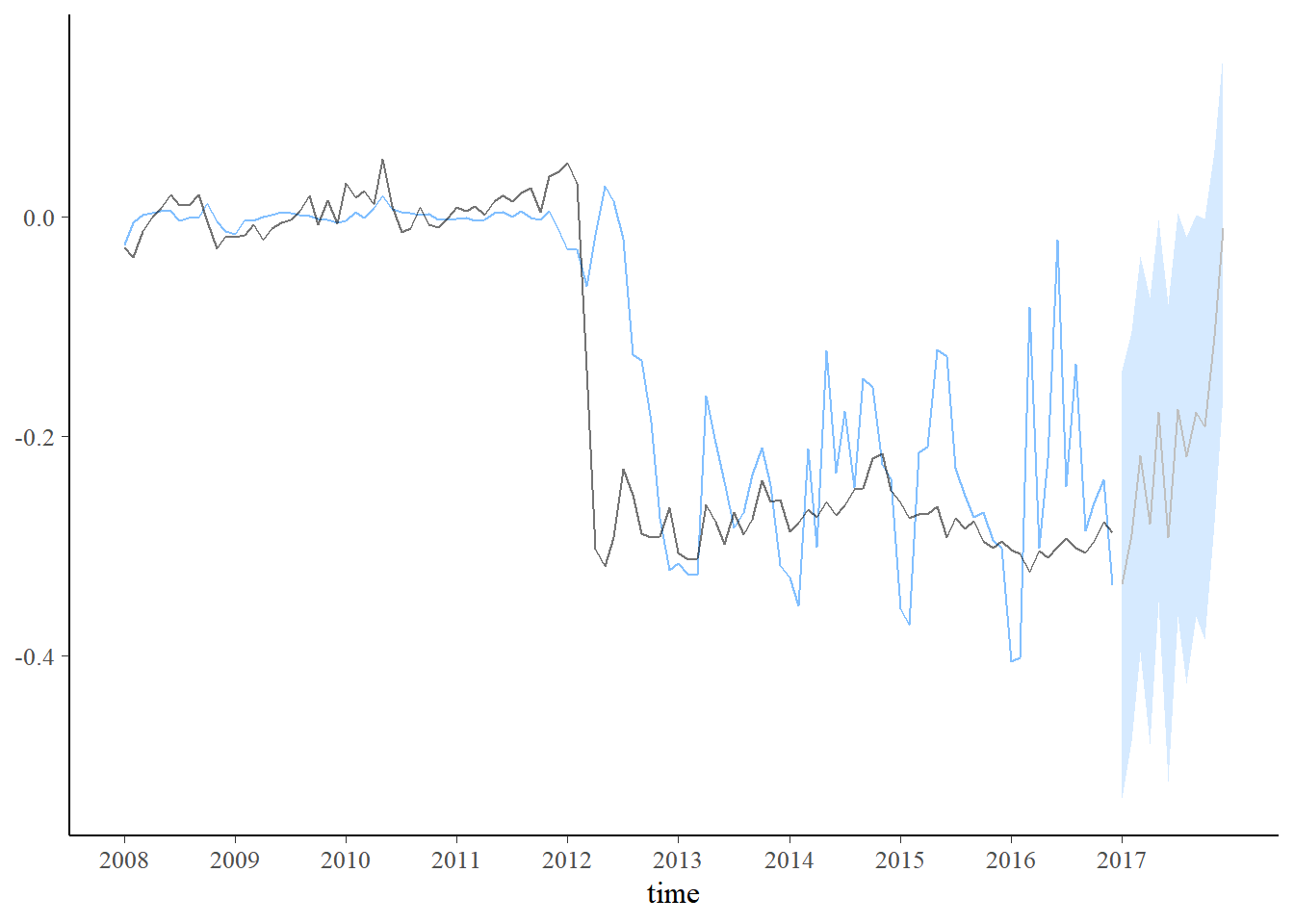
set.seed(666)
new_data <- data.frame(Vendas=seq(dados$Vendas[108]-mAntes[1],-1,length.out=12)+c(0,rnorm(11,0,0.08)))
pred1 <- predict(fit1, new_data)
plot_predict(pred1, alpha=0.8) +
  scale_x_continuous(breaks=seq(1,length(dados$Período)+1,12),labels=c(unique(year(dados$Período)),2017))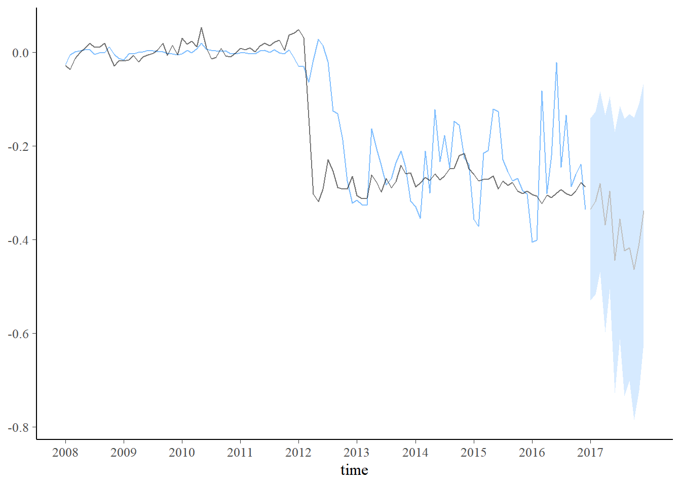
8.5.1.1 Extensões: Efeitos mais suaves e modelos não gaussianos
Ao modelar os coeficientes de regressão como uma passeio aleatório simples, as estimativas posteriores desses coeficientes podem ter grandes variações de curto prazo que podem não ser realistas na prática. Uma maneira de impor mais suavidade às estimativas é alternar dos coeficientes do passeio aleatório para coeficientes de passeio aleatório de segunda ordem integrados: \[\boldsymbol\beta_{t+1} = \boldsymbol\beta_t + \boldsymbol\nu_t\] \[\boldsymbol\nu_{t+1} = \boldsymbol\nu_t + \boldsymbol\eta_t ~,~~ \boldsymbol\eta_t \sim \textit{Normal}_k(0,D)\]
require(walker)
set.seed(666)
fit2 <- dados %>%
  mutate(Vendas=Vendas-mAntes[1],Resistência=Resistência-mAntes[2]) %>%
  walker(data=., formula = Resistência ~ -1+rw2(~ -1+Vendas, beta=c(0,100),
        sigma=c(2,0.0001),nu=c(0,100)),sigma_y_prior=c(2,0.0001), chain=2)
##
## SAMPLING FOR MODEL 'walker_lm' NOW (CHAIN 1).
## Chain 1:
## Chain 1: Gradient evaluation took 0.001 seconds
## Chain 1: 1000 transitions using 10 leapfrog steps per transition would take 10 seconds.
## Chain 1: Adjust your expectations accordingly!
## Chain 1:
## Chain 1:
## Chain 1: Iteration: 1 / 2000 [ 0%] (Warmup)
## Chain 1: Iteration: 200 / 2000 [ 10%] (Warmup)
## Chain 1: Iteration: 400 / 2000 [ 20%] (Warmup)
## Chain 1: Iteration: 600 / 2000 [ 30%] (Warmup)
## Chain 1: Iteration: 800 / 2000 [ 40%] (Warmup)
## Chain 1: Iteration: 1000 / 2000 [ 50%] (Warmup)
## Chain 1: Iteration: 1001 / 2000 [ 50%] (Sampling)
## Chain 1: Iteration: 1200 / 2000 [ 60%] (Sampling)
## Chain 1: Iteration: 1400 / 2000 [ 70%] (Sampling)
## Chain 1: Iteration: 1600 / 2000 [ 80%] (Sampling)
## Chain 1: Iteration: 1800 / 2000 [ 90%] (Sampling)
## Chain 1: Iteration: 2000 / 2000 [100%] (Sampling)
## Chain 1:
## Chain 1: Elapsed Time: 8.11 seconds (Warm-up)
## Chain 1: 7.352 seconds (Sampling)
## Chain 1: 15.462 seconds (Total)
## Chain 1:
##
## SAMPLING FOR MODEL 'walker_lm' NOW (CHAIN 2).
## Chain 2:
## Chain 2: Gradient evaluation took 0.002 seconds
## Chain 2: 1000 transitions using 10 leapfrog steps per transition would take 20 seconds.
## Chain 2: Adjust your expectations accordingly!
## Chain 2:
## Chain 2:
## Chain 2: Iteration: 1 / 2000 [ 0%] (Warmup)
## Chain 2: Iteration: 200 / 2000 [ 10%] (Warmup)
## Chain 2: Iteration: 400 / 2000 [ 20%] (Warmup)
## Chain 2: Iteration: 600 / 2000 [ 30%] (Warmup)
## Chain 2: Iteration: 800 / 2000 [ 40%] (Warmup)
## Chain 2: Iteration: 1000 / 2000 [ 50%] (Warmup)
## Chain 2: Iteration: 1001 / 2000 [ 50%] (Sampling)
## Chain 2: Iteration: 1200 / 2000 [ 60%] (Sampling)
## Chain 2: Iteration: 1400 / 2000 [ 70%] (Sampling)
## Chain 2: Iteration: 1600 / 2000 [ 80%] (Sampling)
## Chain 2: Iteration: 1800 / 2000 [ 90%] (Sampling)
## Chain 2: Iteration: 2000 / 2000 [100%] (Sampling)
## Chain 2:
## Chain 2: Elapsed Time: 7.654 seconds (Warm-up)
## Chain 2: 6.223 seconds (Sampling)
## Chain 2: 13.877 seconds (Total)
## Chain 2: #Default: chain=4, iter=2000, warmup=1000, thin=1
ggpubr::ggarrange(
mcmc_areas(as.matrix(fit2$stanfit), regex_pars = c("sigma_rw2"), prob=0.9),
mcmc_areas(as.matrix(fit2$stanfit), regex_pars = c("sigma_y"), prob=0.9),ncol=1)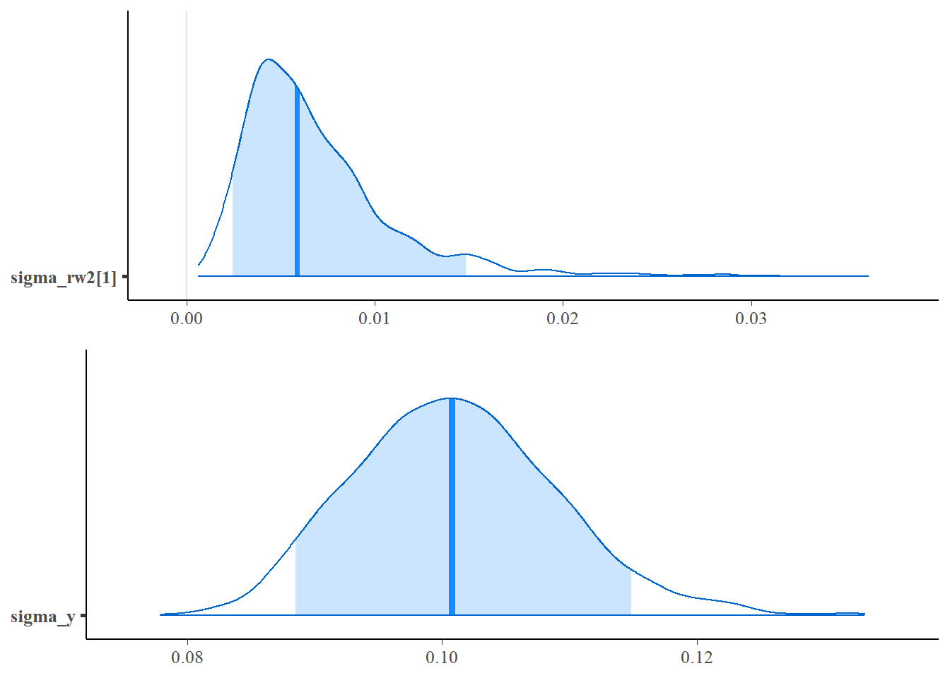
plot_coefs(fit2, scales = "free", alpha=0.8) + theme_bw() +
  scale_x_continuous(breaks=seq(1,length(dados$Período)+1,12),labels=c(unique(year(dados$Período)),2017))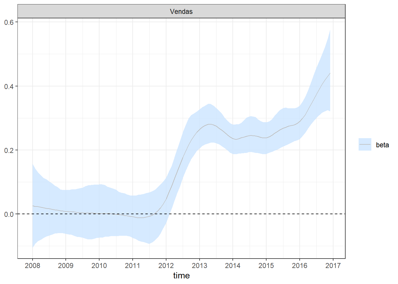
pp_check(fit2, alpha=0.8) + theme_bw() +
  scale_x_continuous(breaks=seq(1,length(dados$Período)+1,12),labels=c(unique(year(dados$Período)),2017))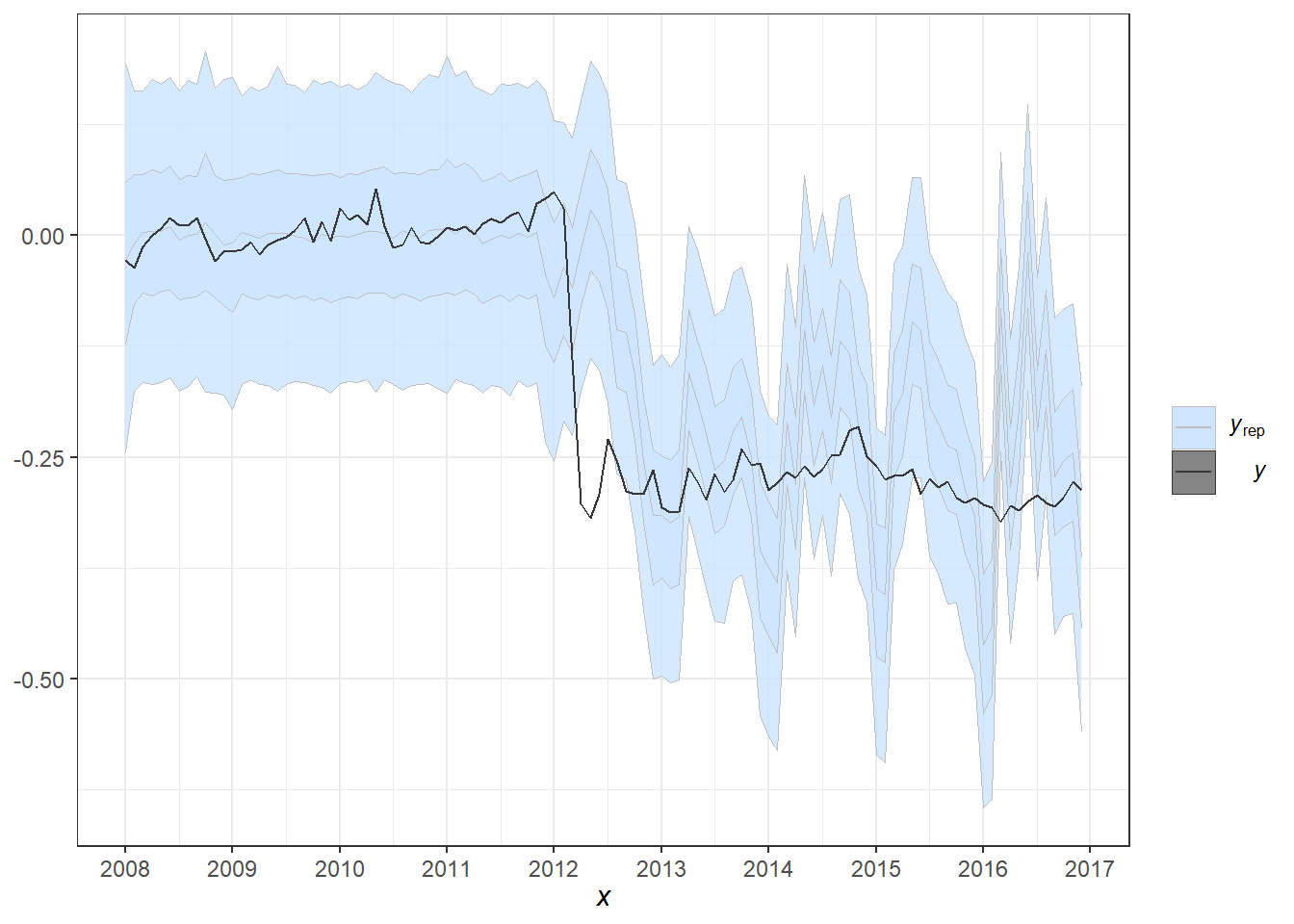
set.seed(666)
new_data <- data.frame(Vendas=seq(dados$Vendas[108]-mAntes[1],-0.2,length.out=12)+c(0,rnorm(11,0,0.08)))
pred2 <- predict(fit2, new_data)
plot_predict(pred2, alpha=0.8) +
  scale_x_continuous(breaks=seq(1,length(dados$Período)+1,12),labels=c(unique(year(dados$Período)),2017))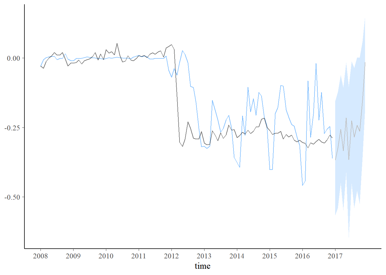
set.seed(666)
new_data <- data.frame(Vendas=seq(dados$Vendas[108]-mAntes[1],-1,length.out=12)+c(0,rnorm(11,0,0.08)))
pred2 <- predict(fit2, new_data)
plot_predict(pred2, alpha=0.8) +
scale_x_continuous(breaks=seq(1,length(dados$Período)+1,12),labels=c(unique(year(dados$Período)),2017))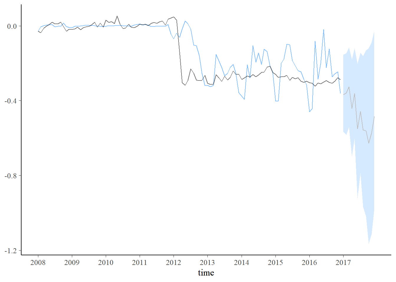 \(~\)
\(~\)
- A função
walker_glmestende o pacote para lidar com observações de com distribuição de Poisson e Binomial, usando a metodologia similar à mencionada acima.
\(~\)
8.5.2 Dados de Covid-19
- Dados de Covid-19: Brasil.io
- Data: dia/mes/ano.
- Casos Novos: novos casos registrados no dia.
- Mortes: mortes registradas no dia.
- Data: dia/mes/ano.
- Dados de Mobilidade: Google
- Data: dia/mes/ano.
- Varejo e Lazer: Tendências de mobilidade de lugares como restaurantes, cafés, shopping centers, parques temáticos, museus, bibliotecas e cinemas.
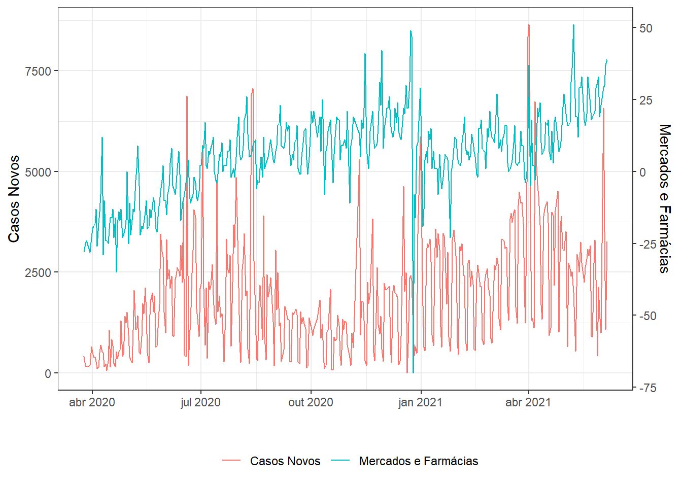
- Mercados e Farmácias: Tendências de mobilidade de lugares como mercados, armazéns de alimentos, feiras, lojas de alimentos gourmet, drogarias e farmácias.
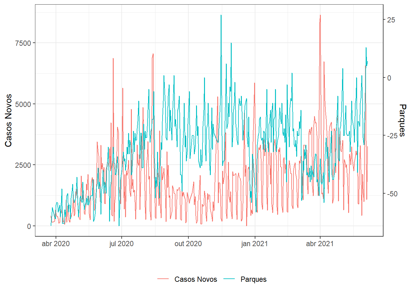
- Parques: Tendências de mobilidade de lugares como parques nacionais, praias públicas, marinas, parques para cães, praças e jardins públicos.
- Transporte: Tendências de mobilidade de lugares como terminais de transporte público, por exemplo, estações de metrô, ônibus e trem.
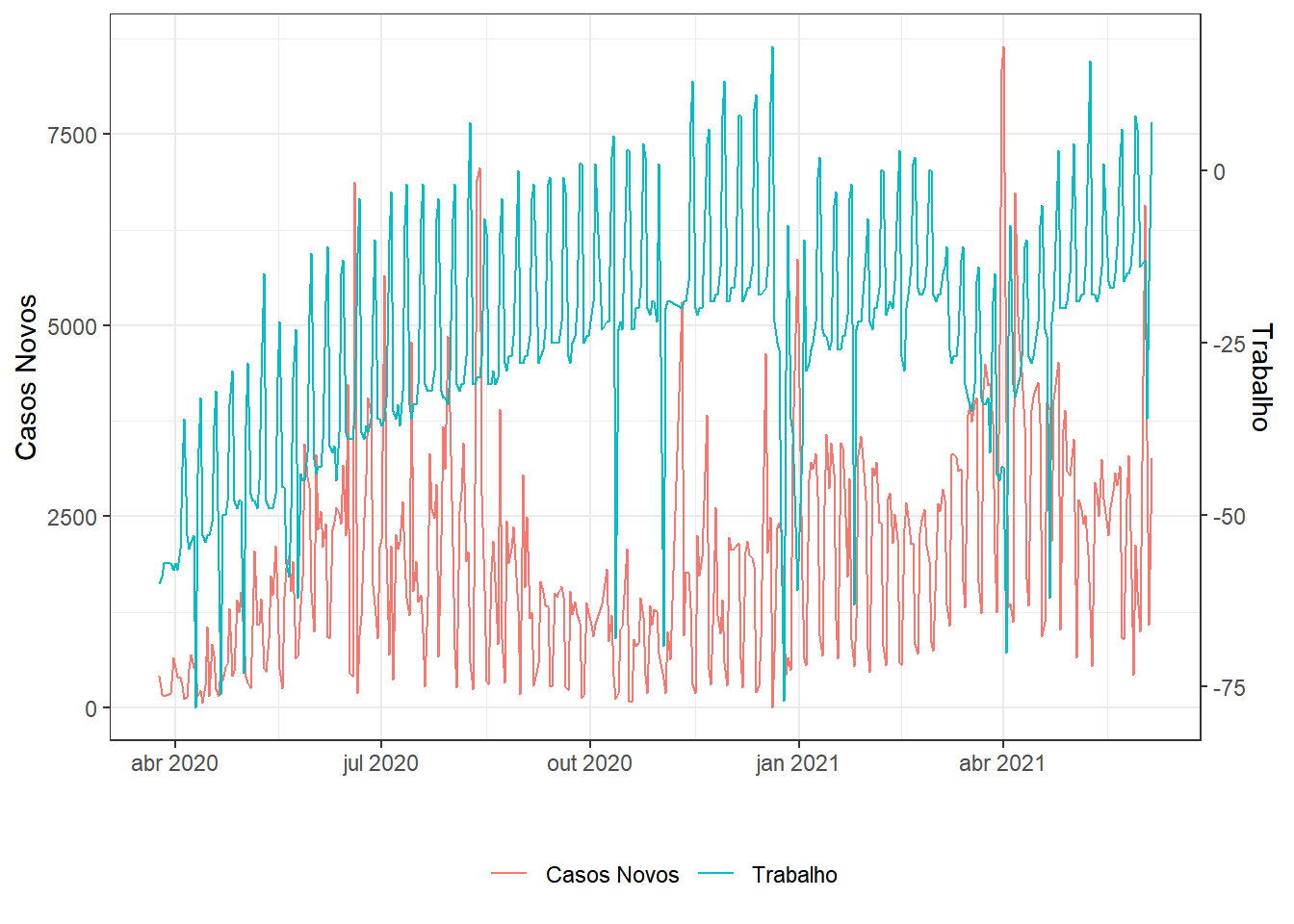
- Trabalho: Tendências de mobilidade de locais de trabalho.
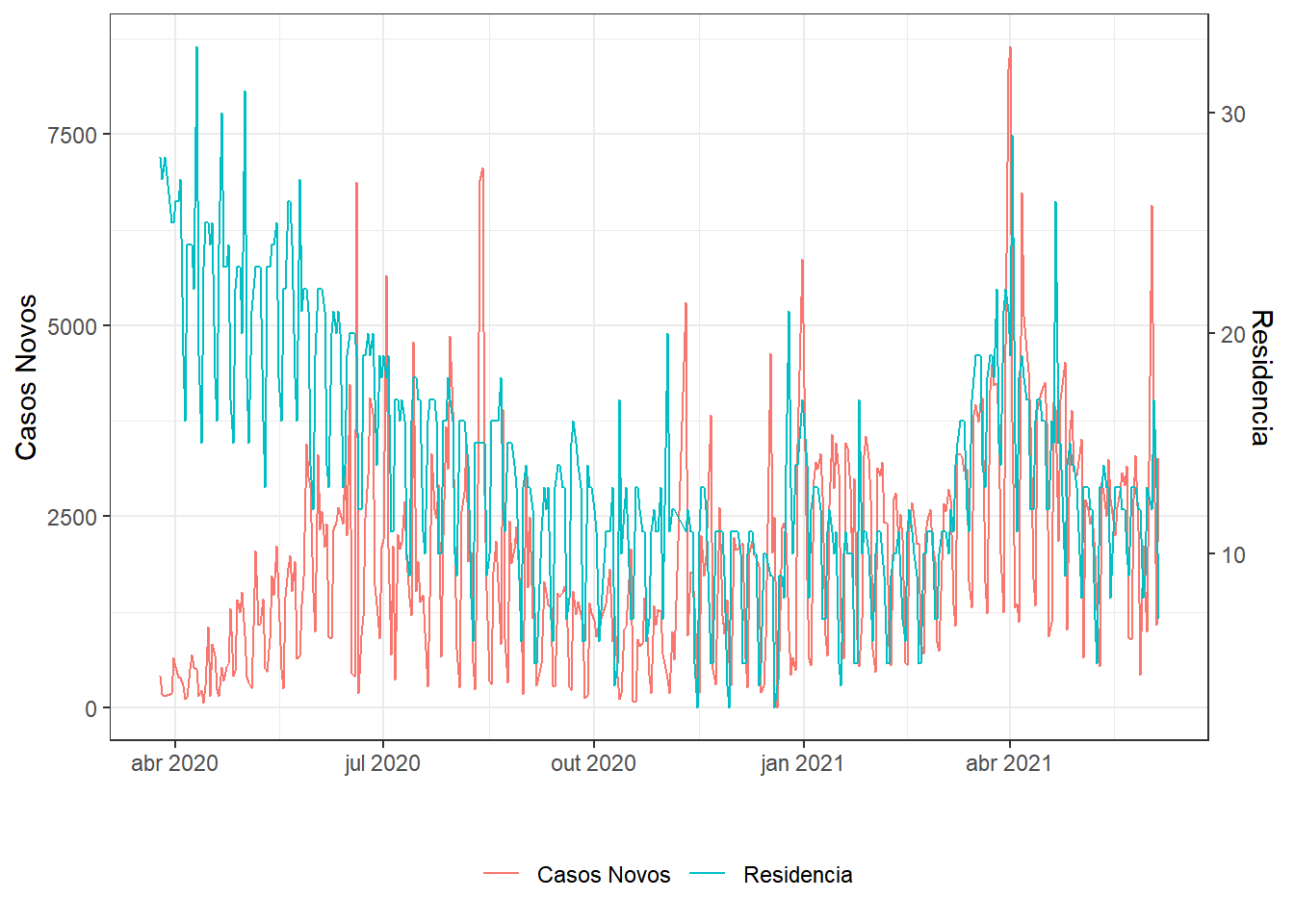
- Residência: Tendências de mobilidade de áreas residenciais.
- Data: dia/mes/ano.
require(walker)
# dados1 = read_csv("./data/covid19-Brasil.io-SPSP.csv") %>%
#   select(epidemiological_week,date,order_for_place,
#          last_available_confirmed,new_confirmed,
#          last_available_confirmed_per_100k_inhabitants,
#          last_available_deaths,new_deaths,
#          last_available_death_rate,estimated_population)
# dados2 = rbind(read_csv("./data/2020_BR_Region_Mobility_Report.csv") %>%
#     filter(sub_region_1=="State of São Paulo",sub_region_2=="São Paulo"),
#    read_csv("./data/2021_BR_Region_Mobility_Report.csv") %>%
#     filter(sub_region_1=="State of São Paulo",sub_region_2=="São Paulo"))%>%
#   select(date, retail_and_recreation_percent_change_from_baseline,
#                grocery_and_pharmacy_percent_change_from_baseline,
#                parks_percent_change_from_baseline,
#                transit_stations_percent_change_from_baseline,
#                workplaces_percent_change_from_baseline,
#                residential_percent_change_from_baseline)
# dados = inner_join(dados1,dados2,by="date")
# write_csv(dados, file="./data/Covid_SPSP.csv")

dados = read_csv("./data/Covid_SPSP.csv")

# Faz gráfico de duas séries temporais ajustando os eixos
# dados é da forma (tempo,série1,série2)
series = function(dados,name1=names(dados)[2],name2=names(dados)[3]){
  # aux para eixo secundário
  aux=(max(dados[[2]])-min(dados[[2]]))/(max(dados[[3]])-min(dados[[3]]))
  dados %>% ggplot(aes(x = dados[[1]])) + theme_bw() +
    geom_line(aes(y = dados[[2]], colour = name1)) +
    geom_line(aes(y = (dados[[3]]-min(dados[[3]]))*aux+min(dados[[2]]), colour = name2)) +
    scale_y_continuous(sec.axis=
      sec_axis(~./aux-min(dados[[2]])/aux+min(dados[[3]]),name=name2)) +
    labs(x="",y=name1,colour="") + theme(legend.position = "bottom")
}

g1=dados %>%
  filter(date>="2020-03-23") %>% # uma semana após início da quarentena
  select(date,new_confirmed,
      retail_and_recreation_percent_change_from_baseline) %>%
  series(.,"Casos Novos","Varejo e Lazer")

g2=dados %>%
  filter(date>="2020-03-23") %>% # uma semana após início da quarentena
  select(date,new_confirmed,
      grocery_and_pharmacy_percent_change_from_baseline) %>%
  series(.,"Casos Novos","Mercados e Farmácias")

g3=dados %>%
  filter(date>="2020-03-23") %>% # uma semana após início da quarentena
  select(date,new_confirmed,
      parks_percent_change_from_baseline) %>%
  series(.,"Casos Novos","Parques")

g4=dados %>%
  filter(date>="2020-03-23") %>% # uma semana após início da quarentena
  select(date,new_confirmed,
      transit_stations_percent_change_from_baseline) %>%
  series(.,"Casos Novos","Transporte")

g5=dados %>%
  filter(date>="2020-03-23") %>% # uma semana após início da quarentena
  select(date,new_confirmed,
      workplaces_percent_change_from_baseline) %>%
  series(.,"Casos Novos","Trabalho")

g6=dados %>%
  filter(date>="2020-03-23") %>% # uma semana após início da quarentena
  select(date,new_confirmed,
      residential_percent_change_from_baseline) %>%
  series(.,"Casos Novos","Residencia")
g1;g2;g3;g4;g5;g6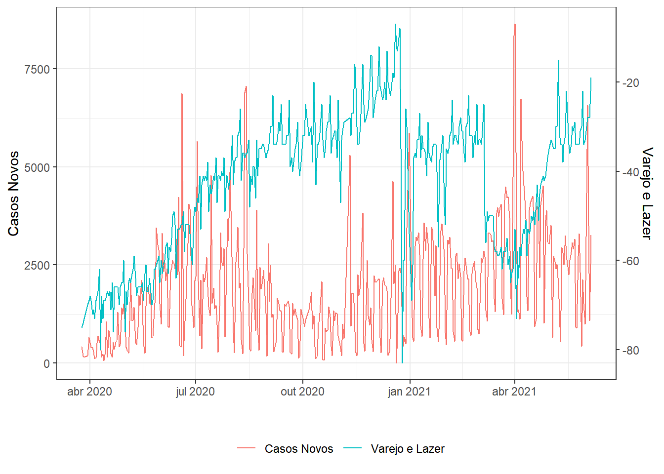

ds =  dados %>%
  mutate(y=new_confirmed,x1=retail_and_recreation_percent_change_from_baseline,x2=grocery_and_pharmacy_percent_change_from_baseline,x3=parks_percent_change_from_baseline,x4=dados$transit_stations_percent_change_from_baseline,x5=workplaces_percent_change_from_baseline, x6=residential_percent_change_from_baseline, t=date, y2=new_deaths) %>%
  arrange(date) %>%
  select(t,y,x1,x2,x3,x4,x5,x6,y2) %>%
  filter(t>="2020-03-23") %>% # uma semana após início da quarentena
  mutate(x=x6-x4)             # "Índice de Mobilidade" (inventei!)

seriesxy=ds %>% select(t,y,x) %>%
  series(.,name1="Casos Novos",name2="Índice de Mobilidade")
seriesxy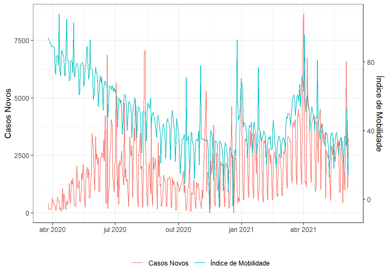
require(walker)
fit1 <- ds %>% #mutate(x=x-mean(x),y=y-mean(y)) %>%
  walker(data=., formula = y ~ -1+rw1(~ 1+x,beta=c(0,100),
    sigma=c(2,0.0001)),sigma_y_prior = c(2,0.0001), chain=1)
##
## SAMPLING FOR MODEL 'walker_lm' NOW (CHAIN 1).
## Chain 1:
## Chain 1: Gradient evaluation took 0.006 seconds
## Chain 1: 1000 transitions using 10 leapfrog steps per transition would take 60 seconds.
## Chain 1: Adjust your expectations accordingly!
## Chain 1:
## Chain 1:
## Chain 1: Iteration: 1 / 2000 [ 0%] (Warmup)
## Chain 1: Iteration: 200 / 2000 [ 10%] (Warmup)
## Chain 1: Iteration: 400 / 2000 [ 20%] (Warmup)
## Chain 1: Iteration: 600 / 2000 [ 30%] (Warmup)
## Chain 1: Iteration: 800 / 2000 [ 40%] (Warmup)
## Chain 1: Iteration: 1000 / 2000 [ 50%] (Warmup)
## Chain 1: Iteration: 1001 / 2000 [ 50%] (Sampling)
## Chain 1: Iteration: 1200 / 2000 [ 60%] (Sampling)
## Chain 1: Iteration: 1400 / 2000 [ 70%] (Sampling)
## Chain 1: Iteration: 1600 / 2000 [ 80%] (Sampling)
## Chain 1: Iteration: 1800 / 2000 [ 90%] (Sampling)
## Chain 1: Iteration: 2000 / 2000 [100%] (Sampling)
## Chain 1:
## Chain 1: Elapsed Time: 43.187 seconds (Warm-up)
## Chain 1: 35.847 seconds (Sampling)
## Chain 1: 79.034 seconds (Total)
## Chain 1: #Default: chain=4, iter=2000, warmup=1000, thin=1
labelx = ds %>% select(t) %>%
mutate(x=seq(1,nrow(ds)),dia1=lubridate::day(t),
labx=lubridate::month(t, label = TRUE)) %>%
filter(dia1==1) %>% select(x,labx) %>%
add_row(x=214,labx="nov",.after=7) %>%
add_row(x=267,labx="jan",.after=9) %>%
add_row(x=c(385,414),labx=c("mai","jun"))
ggpubr::ggarrange(
mcmc_areas(fit1$stanfit,pars = c("sigma_rw1[1]"),prob=0.9),
mcmc_areas(fit1$stanfit,pars = c("sigma_rw1[2]"),prob=0.9),
mcmc_areas(fit1$stanfit,pars = c("sigma_y"),prob=0.9),
ncol=1,align="v")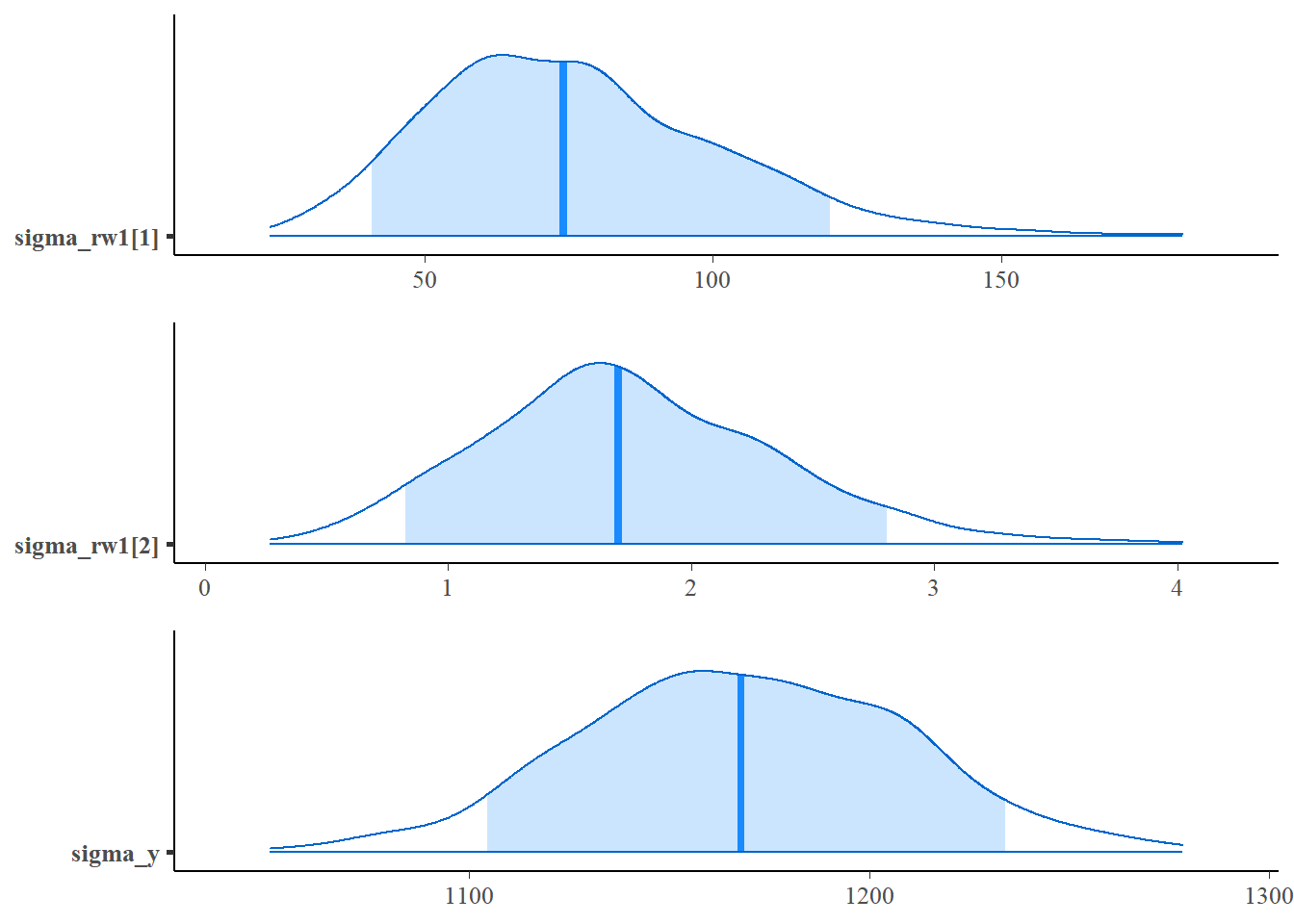
plotcoef=plot_coefs2(fit1,scales="free",alpha=0.8,col=1) + theme_bw() +
  scale_x_continuous(breaks=labelx$x,labels=labelx$labx)
plotcoef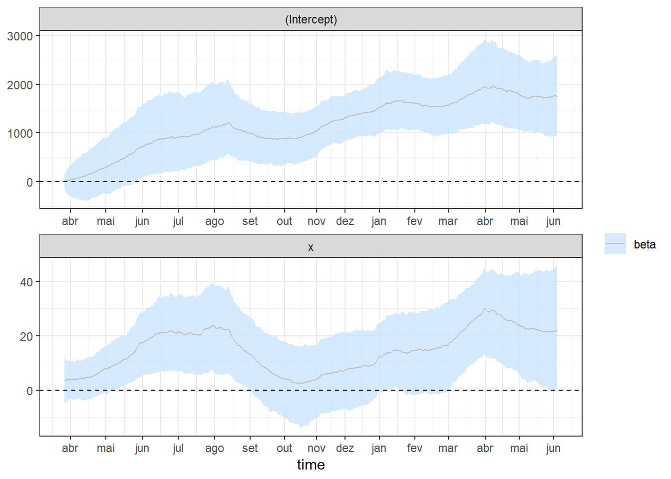
ggpubr::ggarrange(seriesxy,plotcoef,heights=c(1,2),
          ncol = 1, align = "v",common.legend=T,legend="bottom")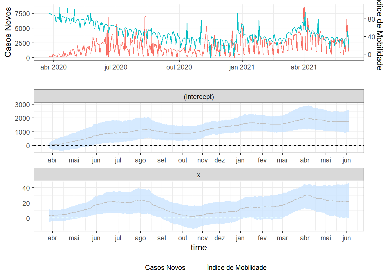
pp_check(fit1, alpha=0.8) + theme_bw() +
  scale_x_continuous(breaks=labelx$x,labels=labelx$labx)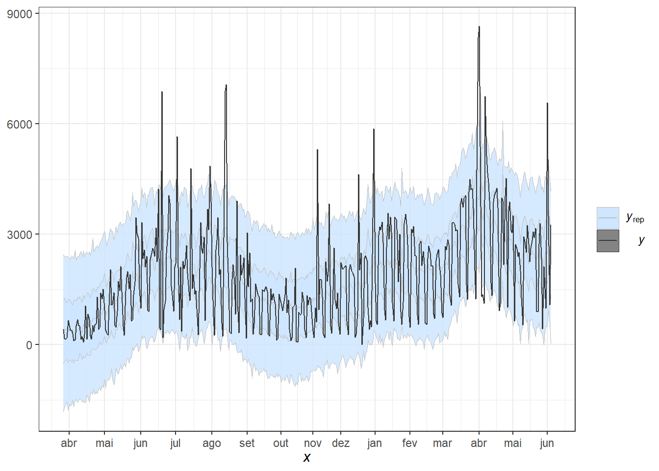
# predição com aumento da taxa de isolamento
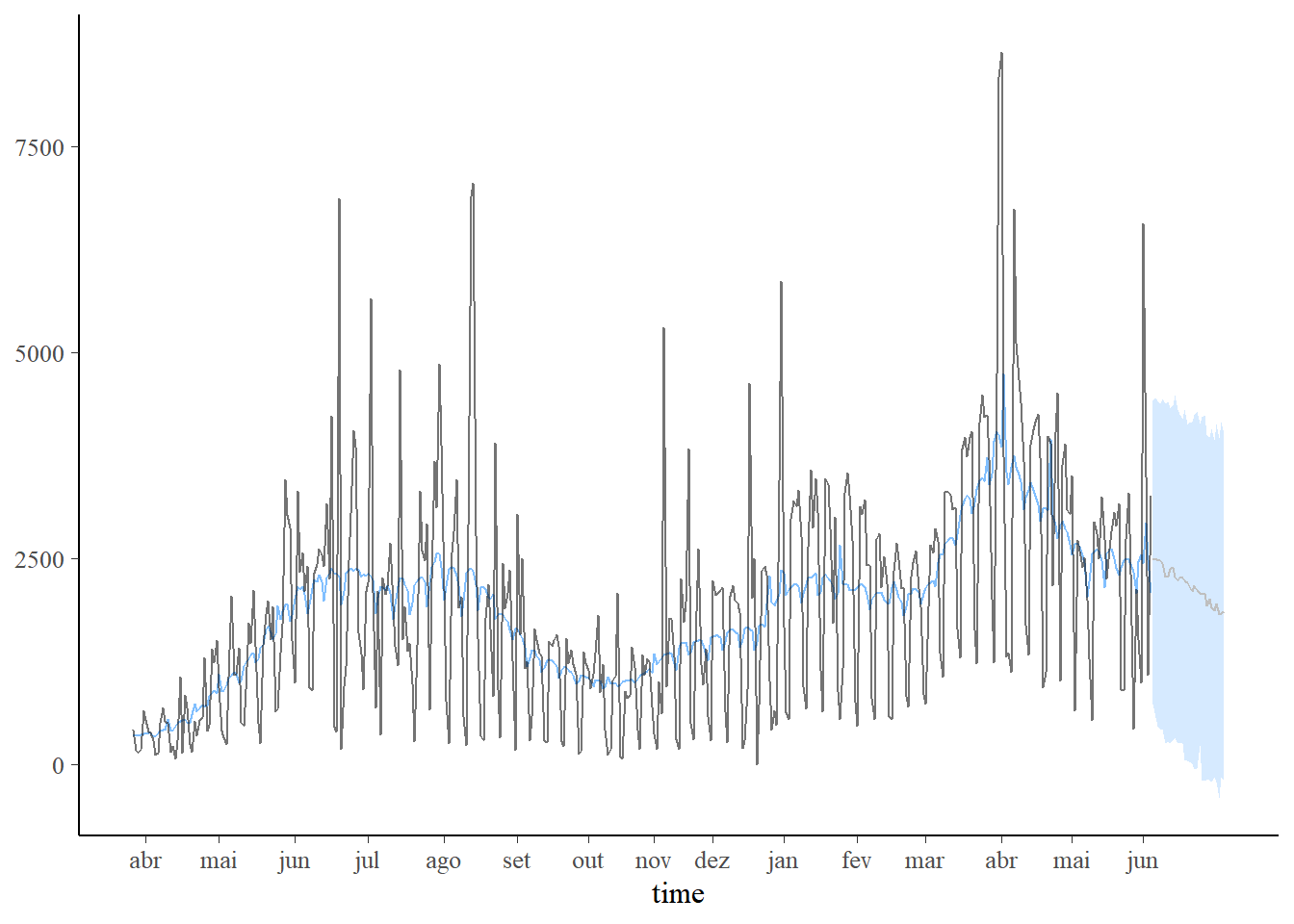
new_data <- data.frame(x=seq(34,64,length.out=30))
pred1 <- predict(fit1, new_data)
plot_predict(pred1, alpha=0.8) +
scale_x_continuous(breaks=labelx$x,labels=labelx$labx)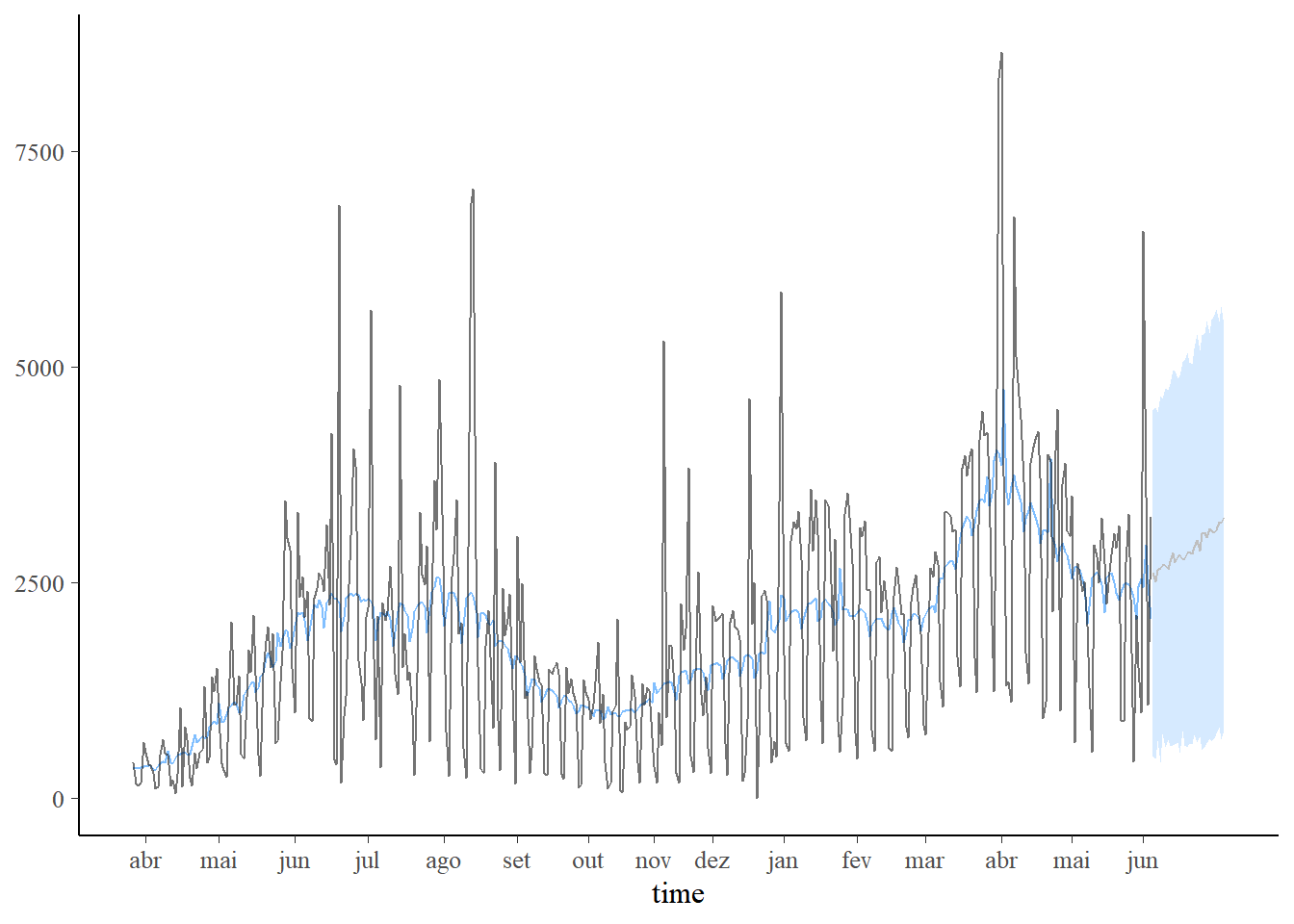
#predição com diminuição da taxa de isolamento
new_data <- data.frame(x=seq(34,4,length.out=30))
pred2 <- predict(fit1, new_data)
plot_predict(pred2, alpha=0.8) +
  scale_x_continuous(breaks=labelx$x,labels=labelx$labx)